A couple weeks ago, we discussed how to perform multi-label classification using Keras and deep learning.
Today, we are going to discuss a more advanced technique called multi-output classification.
So, what’s the difference between the two? And how are you supposed to keep track of all these terms?
While it can be a bit confusing, especially if you are new to studying deep learning, this is how I keep them straight:
- In multi-label classification, your network has only one set of fully-connected layers (i.e., “heads”) at the end of the network responsible for classification.
- But in multi-output classification your network branches at least twice (sometimes more), creating multiple sets of fully-connected heads at the end of the network — your network can then predict a set of class labels for each head, making it possible to learn disjoint label combinations.
You can even combine multi-label classification with multi-output classification so that each fully-connected head can predict multiple outputs!
If this is starting to make your head spin, no worries — I’ve designed today’s tutorial to guide you through multiple output classification with Keras. It’s actually quite easier than it sounds.
That said, this is a more advanced deep learning technique we’re covering today so if you have not already read my first post on Multi-label classification with Keras make sure you do that now.
From there, you’ll be prepared to train your network with multiple loss functions and obtain multiple outputs from the network.
To learn how to use multiple outputs and multiple losses with TensorFlow and Keras, just keep reading!
Keras: Multiple outputs and multiple losses
2020-06-12 Update: This blog post is now TensorFlow 2+ compatible!
In today’s blog post, we are going to learn how to utilize:
- Multiple loss functions
- Multiple outputs
…using the TensorFlow/Keras deep learning library.
As mentioned in the introduction to this tutorial, there is a difference between multi-label and multi-output prediction.
With multi-label classification, we utilize one fully-connected head that can predict multiple class labels.
But with multi-output classification, we have at least two fully-connected heads — each head is responsible for performing a specific classification task.
We can even combine multi-output classification with multi-label classification — in this scenario, each multi-output head would be responsible for computing multiple labels as well!
Your eyes might be starting to gloss over or your might be feeling the first pangs of a headache, so instead of continuing this discussion of multi-output vs. multi-label classification let’s dive into our project. I believe the code presented in this post will help solidify the concept for you.
We’ll start with a review of the dataset we’ll be using to build our multi-output Keras classifier.
From there we’ll implement and train our Keras architecture, FashionNet, which will be used to classify clothing/fashion items using two separate forks in the architecture:
- One fork is responsible for classifying the clothing type of a given input image (ex., shirt, dress, jeans, shoes, etc.).
- And the second fork is responsible for classifying the color of the clothing (black, red, blue, etc.).
Finally, we’ll use our trained network to classify example images and obtain the multi-output classifications.
Let’s go ahead and get started!
The multi-output deep learning dataset
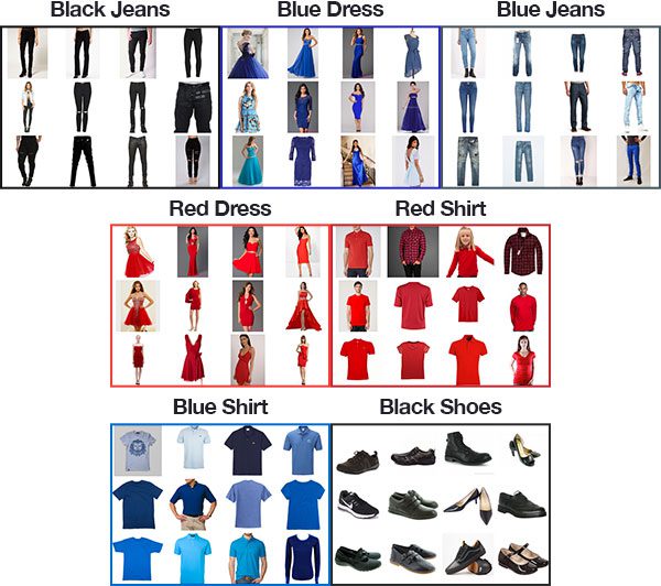
The dataset we’ll be using in today’s Keras multi-output classification tutorial is based on the one from our previous post on multi-label classification with one exception — I’ve added a folder of 358 “black shoes” images.
In total, our dataset consists of 2,525 images across seven color + category combinations, including:
- Black jeans (344 images)
- Black shoes (358 images)
- Blue dress (386 images)
- Blue jeans (356 images)
- Blue shirt (369 images)
- Red dress (380 images)
- Red shirt (332 images)
I created this dataset using the method described in my previous tutorial on How to (quickly) build a deep learning image dataset.
The entire process of downloading the images and manually removing irrelevant images for each of the seven combinations took approximately 30 minutes. When building your own deep learning image datasets, make sure you follow the tutorial linked above — it will give you a huge jumpstart on building your own datasets.
Our goal today is nearly the same as last time — to predict both the color and clothing type…
…with the added twist of being able to predict the clothing type + color of images our network was not trained on.
For example, given the following image of a “black dress” (again, which our network will not be trained on):
Our goal will be to correctly predict both “black” + “dress” for this image.
Configuring your development environment
To configure your system for this tutorial, I recommend following either of these tutorials:
Either tutorial will help you configure you system with all the necessary software for this blog post in a convenient Python virtual environment.
Please note that PyImageSearch does not recommend or support Windows for CV/DL projects.
Our Keras + deep learning project structure
To work through today’s code walkthrough as well as train + test FashionNet on your own images, scroll to to the “Downloads” section and grab the .zip associated with this blog post.
From there, unzip the archive and change directories (cd ) as shown below. Then, utilizing the tree command you can view the files and folders in an organized fashion (pun intended):
$ unzip multi-output-classification.zip
...
$ cd multi-output-classification
$ tree --filelimit 10 --dirsfirst
.
├── dataset
│   ├── black_jeans [344 entries]
│   ├── black_shoes [358 entries]
│   ├── blue_dress [386 entries]
│   ├── blue_jeans [356 entries]
│   ├── blue_shirt [369 entries]
│   ├── red_dress [380 entries]
│   └── red_shirt [332 entries]
├── examples
│   ├── black_dress.jpg
│   ├── black_jeans.jpg
│   ├── blue_shoes.jpg
│   ├── red_shirt.jpg
│   └── red_shoes.jpg
├── output
│   ├── fashion.model
│   ├── category_lb.pickle
│   ├── color_lb.pickle
│   ├── output_accs.png
│   └── output_losses.png
├── pyimagesearch
│   ├── __init__.py
│   └── fashionnet.py
├── train.py
└── classify.py

11 directories, 14 files
Above you can find our project structure, but before we move on, let’s first review the contents.
There are 3 notable Python files:
pyimagesearch/fashionnet.py: Our multi-output classification network file contains the FashionNet architecture class consisting of three methods:build_category_branch,build_color_branch, andbuild. We’ll review these methods in detail in the next section.train.py: This script will train theFashionNetmodel and generate all of the files in the output folder in the process.classify.py: This script loads our trained network and classifies example images using multi-output classification.
We also have 4 top-level directories:
dataset/: Our fashion dataset which was scraped from Bing Image Search using their API. We introduced the dataset in the previous section. To create your own dataset the same way I did, see How to (quickly) build a deep learning image dataset.examples/: We have a handful of example images which we’ll use in conjunction with ourclassify.pyscript in the last section of this blog post.output/: Ourtrain.pyscript generates a handful of output files:fashion.model: Our serialized Keras model.category_lb.pickle: A serializedLabelBinarizerobject for the clothing categories is generated by scikit-learn. This file can be loaded (and labels recalled) by ourclassify.pyscript.color_lb.pickle: ALabelBinarizerobject for colors.output_accs.png: The accuracies training plot image.output_losses.png: The losses training plot image.
pyimagesearch/: This is a Python module containing theFashionNetclass.
A quick review of our multi-output Keras architecture
To perform multi-output prediction with Keras we will be implementing a special network architecture (which I created for the purpose of this blog post) called FashionNet.
The FashionNet architecture contains two special components, including:
- A branch early in the network that splits the network into two “sub-networks” — one responsible for clothing type classification and the other for color classification.
- Two (disjoint) fully-connected heads at the end of the network, each in charge of its respective classification duty.
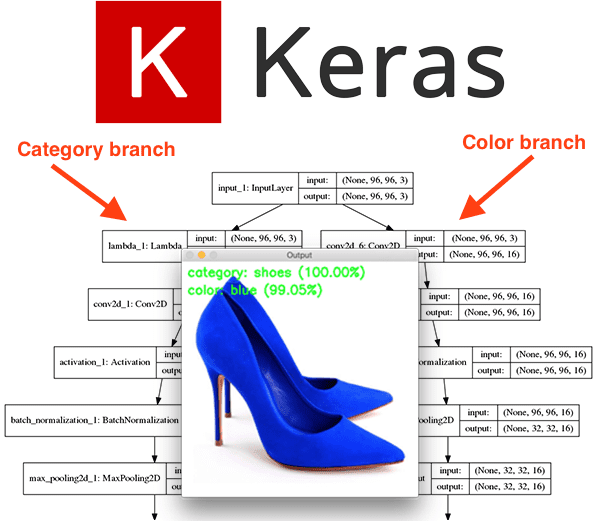
Before we start implementing FashionNet, let’s visualize each of these components, the first being the branching:
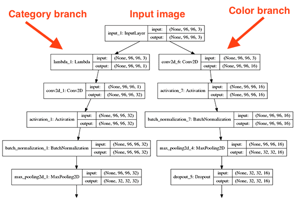
In this network architecture diagram, you can see that our network accepts a 96 x 96 x 3 input image.
We then immediately create two branches:
- The branch on the left is responsible for classifying the clothing category.
- The branch on the right handles classifying the color.
Each branch performs its respective set of convolution, activation, batch normalization, pooling, and dropout operations until we reach the final outputs:
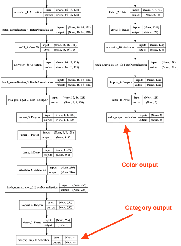
Notice how these sets of fully-connected (FC) heads look like the FC layers from other architectures we’ve examined on this blog — but now there are two of them, each of them responsible for its given classification task.
The branch on the right-hand side of the network is significantly shallower (not as deep) as the left branch. Predicting color is far easier than predicting clothing category and thus the color branch is shallow in comparison.
To see how we can implement such an architecture, let’s move on to our next section.
Implementing our “FashionNet” architecture
Since training a network with multiple outputs using multiple loss functions is more of an advanced technique, I’ll be assuming you understand the fundamentals of CNNs and instead focus on the elements that make multi-output/multi-loss training possible.
If you’re new to the world of deep learning and image classification you should consider working through my book, Deep Learning for Computer Vision with Python, to help you get up to speed.
Ensure you’ve downloaded the files and data from the “Downloads” section before proceeding.
Once you have the downloads in hand, let’s open up fashionnet.py and review:
# import the necessary packages
from tensorflow.keras.models import Model
from tensorflow.keras.layers import BatchNormalization
from tensorflow.keras.layers import Conv2D
from tensorflow.keras.layers import MaxPooling2D
from tensorflow.keras.layers import Activation
from tensorflow.keras.layers import Dropout
from tensorflow.keras.layers import Lambda
from tensorflow.keras.layers import Dense
from tensorflow.keras.layers import Flatten
from tensorflow.keras.layers import Input
import tensorflow as tf
We begin by importing modules from the Keras library and by importing TensorFlow itself.
Since our network consists of two sub-networks, we’ll define two functions responsible for building each respective branch.
The first, build_category_branch , used to classify clothing type, is defined below:
class FashionNet:
	@staticmethod
	def build_category_branch(inputs, numCategories,
		finalAct="softmax", chanDim=-1):
		# utilize a lambda layer to convert the 3 channel input to a
		# grayscale representation
		x = Lambda(lambda c: tf.image.rgb_to_grayscale(c))(inputs)

		# CONV => RELU => POOL
		x = Conv2D(32, (3, 3), padding="same")(x)
		x = Activation("relu")(x)
		x = BatchNormalization(axis=chanDim)(x)
		x = MaxPooling2D(pool_size=(3, 3))(x)
		x = Dropout(0.25)(x)
The build_category_branch function is defined on Lines 16 and 17 with three notable parameters:
inputs: The input volume to our category branch sub-network.numCategories: The number of categories such as “dress”, “shoes”, “jeans”, “shirt”, etc.finalAct: The final activation layer type with the default being a softmax classifier. If you were performing both multi-output and multi-label classification you would want to change this activation to a sigmoid.
Pay close attention to Line 20 where we use a Lambda layer to convert our image from RGB to grayscale.
Why do this?
Well, a dress is a dress regardless of whether it’s red, blue, green, black, or purple, right?
Thus, we decide to throw away any color information and instead focus on the actual structural components in the image, ensuring our network does not learn to jointly associate a particular color with a clothing type.
Note: Lambdas work differently in Python 3.5 and Python 3.6. I trained this model using Python 3.5 so if you just run the classify.py script to test the model with example images with Python 3.6 you may encounter difficulties. If you run into an error related to the Lambda layer, I suggest you either (a) try Python 3.5 or (b) train and classify on Python 3.6. No changes to the code are necessary.
We then proceed to build our CONV => RELU => POOL block with dropout on Lines 23-27. Notice that we are using TensorFlow/Keras’ functional API; we need the functional API to create our branched network structure.
Our first CONV layer has 32 filters with a 3 x 3 kernel and RELU activation (Rectified Linear Unit). We apply batch normalization, max pooling, and 25% dropout.
Dropout is the process of randomly disconnecting nodes from the current layer to the next layer. This process of random disconnects naturally helps the network to reduce overfitting as no one single node in the layer will be responsible for predicting a certain class, object, edge, or corner.
This is followed by our two sets of (CONV => RELU) * 2 => POOL blocks:
		# (CONV => RELU) * 2 => POOL
		x = Conv2D(64, (3, 3), padding="same")(x)
		x = Activation("relu")(x)
		x = BatchNormalization(axis=chanDim)(x)
		x = Conv2D(64, (3, 3), padding="same")(x)
		x = Activation("relu")(x)
		x = BatchNormalization(axis=chanDim)(x)
		x = MaxPooling2D(pool_size=(2, 2))(x)
		x = Dropout(0.25)(x)

		# (CONV => RELU) * 2 => POOL
		x = Conv2D(128, (3, 3), padding="same")(x)
		x = Activation("relu")(x)
		x = BatchNormalization(axis=chanDim)(x)
		x = Conv2D(128, (3, 3), padding="same")(x)
		x = Activation("relu")(x)
		x = BatchNormalization(axis=chanDim)(x)
		x = MaxPooling2D(pool_size=(2, 2))(x)
		x = Dropout(0.25)(x)
The changes in filters, kernels, and pool sizes in this code block work in tandem to progressively reduce the spatial size but increase depth.
Let’s bring it together with a FC => RELU layer:
		# define a branch of output layers for the number of different
		# clothing categories (i.e., shirts, jeans, dresses, etc.)
		x = Flatten()(x)
		x = Dense(256)(x)
		x = Activation("relu")(x)
		x = BatchNormalization()(x)
		x = Dropout(0.5)(x)
		x = Dense(numCategories)(x)
		x = Activation(finalAct, name="category_output")(x)

		# return the category prediction sub-network
		return x
The last activation layer is fully connected and has the same number of neurons/outputs as our numCategories .
Take care to notice that we have named our final activation layer "category_output" on Line 57. This is important as we will reference this layer by name later on in train.py .
Let’s define our second function used to build our multi-output classification network. This one is named build_color_branch , which as the name suggests, is responsible for classifying color in our images:
	@staticmethod
	def build_color_branch(inputs, numColors, finalAct="softmax",
		chanDim=-1):
		# CONV => RELU => POOL
		x = Conv2D(16, (3, 3), padding="same")(inputs)
		x = Activation("relu")(x)
		x = BatchNormalization(axis=chanDim)(x)
		x = MaxPooling2D(pool_size=(3, 3))(x)
		x = Dropout(0.25)(x)

		# CONV => RELU => POOL
		x = Conv2D(32, (3, 3), padding="same")(x)
		x = Activation("relu")(x)
		x = BatchNormalization(axis=chanDim)(x)
		x = MaxPooling2D(pool_size=(2, 2))(x)
		x = Dropout(0.25)(x)

		# CONV => RELU => POOL
		x = Conv2D(32, (3, 3), padding="same")(x)
		x = Activation("relu")(x)
		x = BatchNormalization(axis=chanDim)(x)
		x = MaxPooling2D(pool_size=(2, 2))(x)
		x = Dropout(0.25)(x)
Our parameters to build_color_branch are essentially identical to build_category_branch . We distinguish the number of activations in the final layer with numColors (different from numCategories ).
This time, we won’t apply a Lambda grayscale conversion layer because we are actually concerned about color in this area of the network. If we converted to grayscale we would lose all of our color information!
This branch of the network is significantly more shallow than the clothing category branch because the task at hand is much simpler. All we’re asking our sub-network to accomplish is to classify color — the sub-network does not have to be as deep.
Just like our category branch, we have a second fully connected head. Let’s build the FC => RELU block to finish out:
		# define a branch of output layers for the number of different
		# colors (i.e., red, black, blue, etc.)
		x = Flatten()(x)
		x = Dense(128)(x)
		x = Activation("relu")(x)
		x = BatchNormalization()(x)
		x = Dropout(0.5)(x)
		x = Dense(numColors)(x)
		x = Activation(finalAct, name="color_output")(x)

		# return the color prediction sub-network
		return x
To distinguish the final activation layer for the color branch, I’ve provided the name="color_output" keyword argument on Line 94. We’ll refer to the name in the training script.
Our final step for building FashionNet is to put our two branches together and build the final architecture:
	@staticmethod
	def build(width, height, numCategories, numColors,
		finalAct="softmax"):
		# initialize the input shape and channel dimension (this code
		# assumes you are using TensorFlow which utilizes channels
		# last ordering)
		inputShape = (height, width, 3)
		chanDim = -1

		# construct both the "category" and "color" sub-networks
		inputs = Input(shape=inputShape)
		categoryBranch = FashionNet.build_category_branch(inputs,
			numCategories, finalAct=finalAct, chanDim=chanDim)
		colorBranch = FashionNet.build_color_branch(inputs,
			numColors, finalAct=finalAct, chanDim=chanDim)

		# create the model using our input (the batch of images) and
		# two separate outputs -- one for the clothing category
		# branch and another for the color branch, respectively
		model = Model(
			inputs=inputs,
			outputs=[categoryBranch, colorBranch],
			name="fashionnet")

		# return the constructed network architecture
		return model
Our build function is defined on Line 100 and has 5 self-explanatory parameters.
The build function makes an assumption that we’re using TensorFlow and channels last ordering. This is made clear on Line 105 where our inputShape tuple is explicitly ordered (height, width, 3) , where the 3 represents the RGB channels.
If you would like to use a backend other than TensorFlow you’ll need to modify the code to: (1) correctly the proper channel ordering for your backend and (2) implement a custom layer to handle the RGB to grayscale conversion.
From there, we define the two branches of the network (Lines 110-113) and then put them together in a Model (Lines 118-121).
The key takeaway is that our branches have one common input, but two different outputs (the clothing type and color classifications).
Implementing the multi-output and multi-loss training script
Now that we’ve implemented our FashionNet architecture, let’s train it!
When you’re ready, open up train.py and let’s dive in:
# set the matplotlib backend so figures can be saved in the background
import matplotlib
matplotlib.use("Agg")

# import the necessary packages
from tensorflow.keras.optimizers import Adam
from tensorflow.keras.preprocessing.image import img_to_array
from sklearn.preprocessing import LabelBinarizer
from sklearn.model_selection import train_test_split
from pyimagesearch.fashionnet import FashionNet
from imutils import paths
import matplotlib.pyplot as plt
import numpy as np
import argparse
import random
import pickle
import cv2
import os
We begin by importing necessary packages for the script.
From there we parse our command line arguments:
# construct the argument parser and parse the arguments
ap = argparse.ArgumentParser()
ap.add_argument("-d", "--dataset", required=True,
	help="path to input dataset (i.e., directory of images)")
ap.add_argument("-m", "--model", required=True,
	help="path to output model")
ap.add_argument("-l", "--categorybin", required=True,
	help="path to output category label binarizer")
ap.add_argument("-c", "--colorbin", required=True,
	help="path to output color label binarizer")
ap.add_argument("-p", "--plot", type=str, default="output",
	help="base filename for generated plots")
args = vars(ap.parse_args())
We’ll see how to run the training script soon. For now, just know that --dataset is the input file path to our dataset and --model , --categorybin , --colorbin are all three output file paths.
Optionally, you may specify a base filename for the generated accuracy/loss plots using the --plot argument. I’ll point out these command line arguments again when we encounter them in the script. If Lines 21-32 look greek to you, please see my argparse + command line arguments blog post.
Now, let’s establish four important training variables:
# initialize the number of epochs to train for, initial learning rate,
# batch size, and image dimensions
EPOCHS = 50
INIT_LR = 1e-3
BS = 32
IMAGE_DIMS = (96, 96, 3)
We’re setting the following variables on Lines 36-39:
EPOCHS: The number of epochs is set to50. Through experimentation I found that50epochs yields a model that has low loss and has not overfitted to the training set (or not overfitted as best as we can).INIT_LR: Our initial learning rate is set to0.001. The learning rate controls the “step” we make along the gradient. Smaller values indicate smaller steps and larger values indicate bigger steps. We’ll see soon that we’re going to use the Adam optimizer while progressively reducing the learning rate over time.BS: We’ll be training our network in batch sizes of32.IMAGE_DIMS: All input images will be resized to96 x 96with3channels (RGB). We are training with these dimensions and our network architecture input dimensions reflect these as well. When we test our network with example images in a later section, the testing dimensions must match the training dimensions.
Our next step is to grab our image paths and randomly shuffle them. We’ll also initialize lists to hold the images themselves as well as the clothing category and color, respectively:
# grab the image paths and randomly shuffle them
print("[INFO] loading images...")
imagePaths = sorted(list(paths.list_images(args["dataset"])))
random.seed(42)
random.shuffle(imagePaths)

# initialize the data, clothing category labels (i.e., shirts, jeans,
# dresses, etc.) along with the color labels (i.e., red, blue, etc.)
data = []
categoryLabels = []
colorLabels = []
And subsequently, we’ll loop over the imagePaths , preprocess, and populate the data , categoryLabels , and colorLabels lists:
# loop over the input images
for imagePath in imagePaths:
	# load the image, pre-process it, and store it in the data list
	image = cv2.imread(imagePath)
	image = cv2.resize(image, (IMAGE_DIMS[1], IMAGE_DIMS[0]))
	image = cv2.cvtColor(image, cv2.COLOR_BGR2RGB)
	image = img_to_array(image)
	data.append(image)

	# extract the clothing color and category from the path and
	# update the respective lists
	(color, cat) = imagePath.split(os.path.sep)[-2].split("_")
	categoryLabels.append(cat)
	colorLabels.append(color)
We begin looping over our imagePaths on Line 54.
Inside the loop, we load and resize the image to the IMAGE_DIMS . We also convert our image from BGR ordering to RGB. Why do we do this conversion? Recall back to our FashionNet class in the build_category_branch function, where we used TensorFlow’s rgb_to_grayscale conversion in a Lambda function/layer. Because of this, we first convert to RGB on Line 58, and eventually append the preprocessed image to the data list.
Next, still inside of the loop, we extract both the color and category labels from the directory name where the current image resides (Line 64).
To see this in action, just fire up Python in your terminal, and provide a sample imagePath to experiment with like so:
$ python
>>> import os
>>> imagePath = "dataset/red_dress/00000000.jpg"
>>> (color, cat) = imagePath.split(os.path.sep)[-2].split("_")
>>> color
'red'
>>> cat
'dress'
You can of course organize your directory structure any way you wish (but you will have to modify the code). My two favorite methods include (1) using subdirectories for each label or (2) storing all images in a single directory and then creating a CSV or JSON file to map image filenames to their labels.
Let’s convert the three lists to NumPy arrays, binarize the labels, and partition the data into training and testing splits:
# scale the raw pixel intensities to the range [0, 1] and convert to
# a NumPy array
data = np.array(data, dtype="float") / 255.0
print("[INFO] data matrix: {} images ({:.2f}MB)".format(
	len(imagePaths), data.nbytes / (1024 * 1000.0)))

# convert the label lists to NumPy arrays prior to binarization
categoryLabels = np.array(categoryLabels)
colorLabels = np.array(colorLabels)

# binarize both sets of labels
print("[INFO] binarizing labels...")
categoryLB = LabelBinarizer()
colorLB = LabelBinarizer()
categoryLabels = categoryLB.fit_transform(categoryLabels)
colorLabels = colorLB.fit_transform(colorLabels)

# partition the data into training and testing splits using 80% of
# the data for training and the remaining 20% for testing
split = train_test_split(data, categoryLabels, colorLabels,
	test_size=0.2, random_state=42)
(trainX, testX, trainCategoryY, testCategoryY,
	trainColorY, testColorY) = split
Our last preprocessing step — converting to a NumPy array and scaling raw pixel intensities to [0, 1] — can be performed in one swoop on Line 70.
We also convert the categoryLabels and colorLabels to NumPy arrays while we’re at it (Lines 75 and 76). This is necessary as in our next we’re going to binarize the labels using scikit-learn’s LabelBinarizer which we previously imported (Lines 80-83). Since our network has two separate branches, we can use two independent label binarizers — this is different from multi-label classification where we used the MultiLabelBinarizer (also from scikit-learn).
Next, we perform a typical 80% training/20% testing split on our dataset (Lines 87-96).
Let’s build the network, define our independent losses, and compile our model:
# initialize our FashionNet multi-output network
model = FashionNet.build(96, 96,
	numCategories=len(categoryLB.classes_),
	numColors=len(colorLB.classes_),
	finalAct="softmax")

# define two dictionaries: one that specifies the loss method for
# each output of the network along with a second dictionary that
# specifies the weight per loss
losses = {
	"category_output": "categorical_crossentropy",
	"color_output": "categorical_crossentropy",
}
lossWeights = {"category_output": 1.0, "color_output": 1.0}

# initialize the optimizer and compile the model
print("[INFO] compiling model...")
opt = Adam(lr=INIT_LR, decay=INIT_LR / EPOCHS)
model.compile(optimizer=opt, loss=losses, loss_weights=lossWeights,
	metrics=["accuracy"])
On Lines 93-96, we instantiate our multi-output FashionNet model. We dissected the parameters when we created the FashionNet class and build function therein, so be sure to take a look at the values we’re actually providing here.
Next, we need to define two losses for each of the fully-connected heads (Lines 101-104).
Defining multiple losses is accomplished with a dictionary using the names of each of the branch activation layers — this is why we named our output layers in the FashionNet implementation! Each loss will use categorical cross-entropy, the standard loss method used when training networks for classification with > 2 classes.
We also define equal lossWeights in a separate dictionary (same name keys with equal values) on Line 105. In your particular application, you may wish to weight one loss more heavily than the other.
Now that we’ve instantiated our model and created our losses + lossWeights dictionaries, let’s initialize the Adam optimizer with learning rate decay (Line 109) and compile our model (Lines 110 and 111).
Our next block simply kicks off the training process:
# train the network to perform multi-output classification
H = model.fit(x=trainX,
	y={"category_output": trainCategoryY, "color_output": trainColorY},
	validation_data=(testX,
		{"category_output": testCategoryY, "color_output": testColorY}),
	epochs=EPOCHS,
	verbose=1)

# save the model to disk
print("[INFO] serializing network...")
model.save(args["model"], save_format="h5")
2020-06-12 Update: Note that for TensorFlow 2.0+ we recommend explicitly setting the save_format="h5" (HDF5 format).
Recall back to Lines 87-90 where we split our data into training (trainX ) and testing (testX ). On Lines 114-119 we launch the training process while providing the data. Take note on Line 115 where we pass in the labels as a dictionary. The same goes for Lines 116 and 117 where we pass in a 2-tuple for the validation data. Passing in the training and validation labels in this manner is a requirement when performing multi-output classification with Keras. We need to instruct Keras which set of target labels corresponds to which output branch of the network.
Using our command line argument (args["model"] ), we save the serialized model to disk for future recall.
We’ll also do the same to save our label binarizers as serialized pickle files:
# save the category binarizer to disk
print("[INFO] serializing category label binarizer...")
f = open(args["categorybin"], "wb")
f.write(pickle.dumps(categoryLB))
f.close()

# save the color binarizer to disk
print("[INFO] serializing color label binarizer...")
f = open(args["colorbin"], "wb")
f.write(pickle.dumps(colorLB))
f.close()
Using the command line argument paths (args["categorybin"] and args["colorbin"] ) we write both of our label binarizers (categoryLB and colorLB ) to serialized pickle files on disk.
From there it’s all about plotting results in this script:
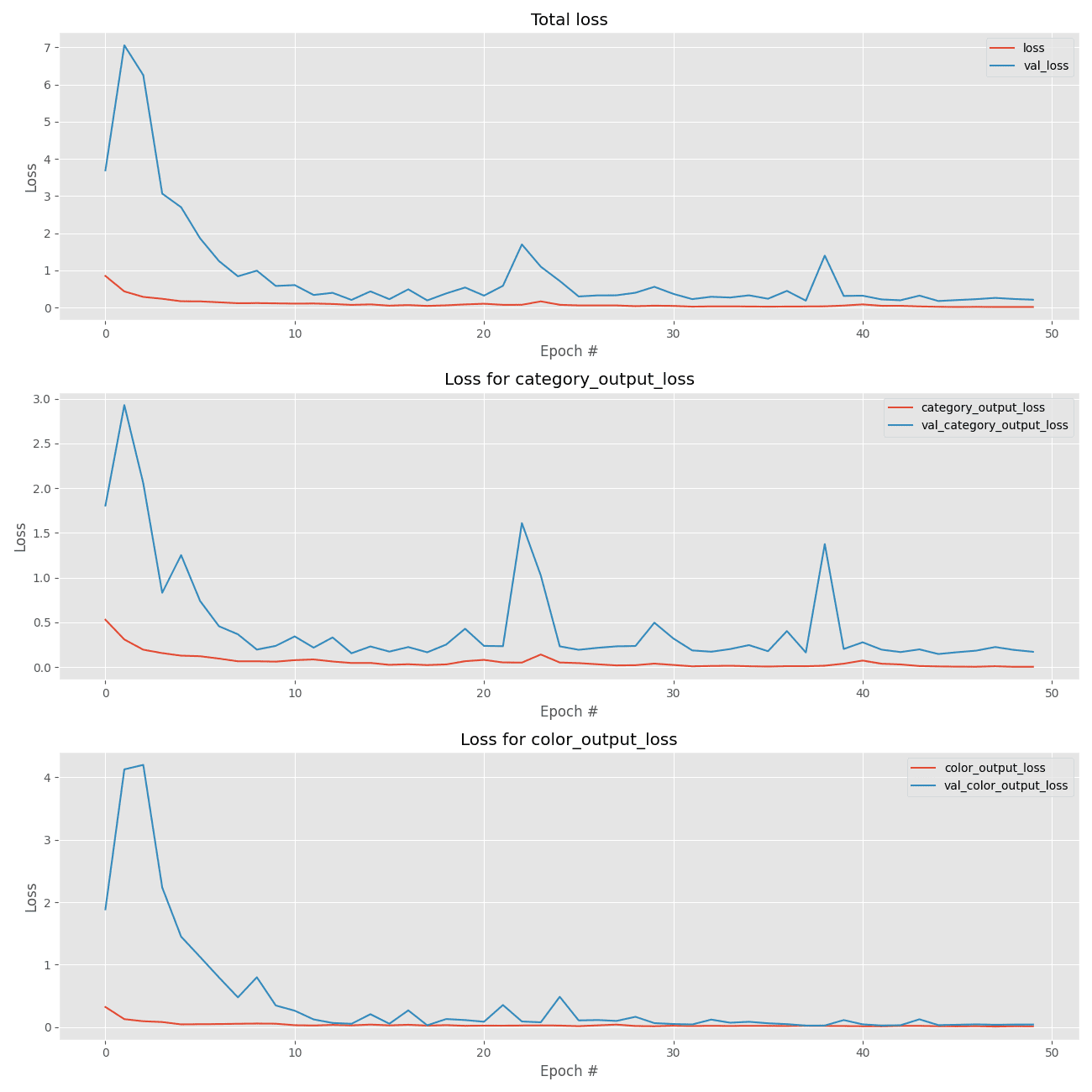
# plot the total loss, category loss, and color loss
lossNames = ["loss", "category_output_loss", "color_output_loss"]
plt.style.use("ggplot")
(fig, ax) = plt.subplots(3, 1, figsize=(13, 13))

# loop over the loss names
for (i, l) in enumerate(lossNames):
	# plot the loss for both the training and validation data
	title = "Loss for {}".format(l) if l != "loss" else "Total loss"
	ax[i].set_title(title)
	ax[i].set_xlabel("Epoch #")
	ax[i].set_ylabel("Loss")
	ax[i].plot(np.arange(0, EPOCHS), H.history[l], label=l)
	ax[i].plot(np.arange(0, EPOCHS), H.history["val_" + l],
		label="val_" + l)
	ax[i].legend()

# save the losses figure
plt.tight_layout()
plt.savefig("{}_losses.png".format(args["plot"]))
plt.close()
The above code block is responsible for plotting the loss history for each of the loss functions on separate but stacked plots, including:
- Total loss
- Loss for the category output
- Loss for the color output
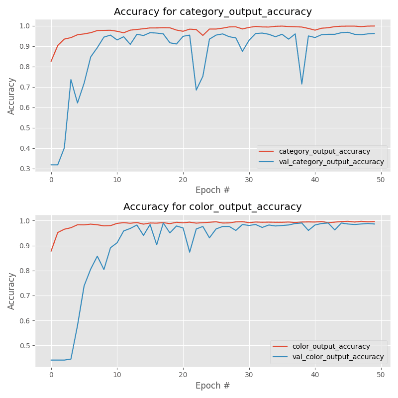
Similarly, we’ll plot the accuracies in a separate image file:
# create a new figure for the accuracies
accuracyNames = ["category_output_accuracy", "color_output_accuracy"]
plt.style.use("ggplot")
(fig, ax) = plt.subplots(2, 1, figsize=(8, 8))

# loop over the accuracy names
for (i, l) in enumerate(accuracyNames):
	# plot the loss for both the training and validation data
	ax[i].set_title("Accuracy for {}".format(l))
	ax[i].set_xlabel("Epoch #")
	ax[i].set_ylabel("Accuracy")
	ax[i].plot(np.arange(0, EPOCHS), H.history[l], label=l)
	ax[i].plot(np.arange(0, EPOCHS), H.history["val_" + l],
		label="val_" + l)
	ax[i].legend()

# save the accuracies figure
plt.tight_layout()
plt.savefig("{}_accs.png".format(args["plot"]))
plt.close()
2020-06-12 Update: In order for this plotting snippet to be TensorFlow 2+ compatible the H.history dictionary keys are updated to fully spell out “accuracy” sans “acc” (i.e., H.history["category_output_accuracy"] and H.history["color_output_accuracy"]). It is semi-confusing that “val” is not spelled out as “validation”; we have to learn to love and live with the API and always remember that it is a work in progress that many developers around the world contribute to.
Our category accuracy and color accuracy plots are best viewed separately, so they are stacked as separate plots in one image.
Training the multi-output/multi-loss Keras model
Be sure to use the “Downloads” section of this blog post to grab the code and dataset.
Don’t forget: I used Python 3.7 to train the network included in the download for this tutorial. As long as you stay consistent (Python 3.5+) you shouldn’t have a problem with the Lambda implementation inconsistency. You can probably even run Python 2.7 (I haven’t tested this).
Open up terminal. Then paste the following command to kick off the training process (if you don’t have a GPU, you’ll want to grab a beer as well):
$ python train.py --dataset dataset --model output/fashion.model \
	--categorybin output/category_lb.pickle --colorbin output/color_lb.pickle
Using TensorFlow backend.
[INFO] loading images...
[INFO] data matrix: 2521 images (544.54MB)
[INFO] loading images...
[INFO] data matrix: 2521 images (544.54MB)
[INFO] binarizing labels...
[INFO] compiling model...
Epoch 1/50
63/63 [==============================] - 1s 20ms/step - loss: 0.8523 - category_output_loss: 0.5301 - color_output_loss: 0.3222 - category_output_accuracy: 0.8264 - color_output_accuracy: 0.8780 - val_loss: 3.6909 - val_category_output_loss: 1.8052 - val_color_output_loss: 1.8857 - val_category_output_accuracy: 0.3188 - val_color_output_accuracy: 0.4416
Epoch 2/50
63/63 [==============================] - 1s 14ms/step - loss: 0.4367 - category_output_loss: 0.3092 - color_output_loss: 0.1276 - category_output_accuracy: 0.9033 - color_output_accuracy: 0.9519 - val_loss: 7.0533 - val_category_output_loss: 2.9279 - val_color_output_loss: 4.1254 - val_category_output_accuracy: 0.3188 - val_color_output_accuracy: 0.4416
Epoch 3/50
63/63 [==============================] - 1s 14ms/step - loss: 0.2892 - category_output_loss: 0.1952 - color_output_loss: 0.0940 - category_output_accuracy: 0.9350 - color_output_accuracy: 0.9653 - val_loss: 6.2512 - val_category_output_loss: 2.0540 - val_color_output_loss: 4.1972 - val_category_output_accuracy: 0.4020 - val_color_output_accuracy: 0.4416
...
Epoch 48/50
63/63 [==============================] - 1s 14ms/step - loss: 0.0189 - category_output_loss: 0.0106 - color_output_loss: 0.0083 - category_output_accuracy: 0.9960 - color_output_accuracy: 0.9970 - val_loss: 0.2625 - val_category_output_loss: 0.2250 - val_color_output_loss: 0.0376 - val_category_output_accuracy: 0.9564 - val_color_output_accuracy: 0.9861
Epoch 49/50
63/63 [==============================] - 1s 14ms/step - loss: 0.0190 - category_output_loss: 0.0041 - color_output_loss: 0.0148 - category_output_accuracy: 0.9985 - color_output_accuracy: 0.9950 - val_loss: 0.2333 - val_category_output_loss: 0.1927 - val_color_output_loss: 0.0406 - val_category_output_accuracy: 0.9604 - val_color_output_accuracy: 0.9881
Epoch 50/50
63/63 [==============================] - 1s 14ms/step - loss: 0.0188 - category_output_loss: 0.0046 - color_output_loss: 0.0142 - category_output_accuracy: 0.9990 - color_output_accuracy: 0.9960 - val_loss: 0.2140 - val_category_output_loss: 0.1719 - val_color_output_loss: 0.0421 - val_category_output_accuracy: 0.9624 - val_color_output_accuracy: 0.9861
[INFO] serializing network...
[INFO] serializing category label binarizer...
[INFO] serializing color label binarizer...
For our category output we obtained:
- 99.90% accuracy on the training set
- 96.24% accuracy on the testing set
And for the color output we reached:
- 99.60% accuracy on the training set
- 98.61% accuracy on the testing set
Below you can find the plots for each of our multiple losses:
As well as our multiple accuracies:
Further accuracy can likely be obtained by applying data augmentation (covered in my book, Deep Learning for Computer Vision with Python).
Implementing a multi-output classification script
Now that we have trained our network, let’s learn how to apply it to input images not part of our training set.
Open up classify.py and insert the following code:
# import the necessary packages
from tensorflow.keras.preprocessing.image import img_to_array
from tensorflow.keras.models import load_model
import tensorflow as tf
import numpy as np
import argparse
import imutils
import pickle
import cv2
First, we import our required packages followed by parsing command line arguments:
# construct the argument parser and parse the arguments
ap = argparse.ArgumentParser()
ap.add_argument("-m", "--model", required=True,
	help="path to trained model model")
ap.add_argument("-l", "--categorybin", required=True,
	help="path to output category label binarizer")
ap.add_argument("-c", "--colorbin", required=True,
	help="path to output color label binarizer")
ap.add_argument("-i", "--image", required=True,
	help="path to input image")
args = vars(ap.parse_args())
We have four command line arguments which are required to make this script run in your terminal:
--model: The path to the serialized model file we just trained (an output of our previous script).--categorybin: The path to the category label binarizer (an output of our previous script).--colorbin: The path to the color label binarizer (an output of our previous script).--image: Our test image file path — this image will come from ourexamples/directory.
From there, we load our image and preprocess it:
# load the image
image = cv2.imread(args["image"])
output = imutils.resize(image, width=400)
image = cv2.cvtColor(image, cv2.COLOR_BGR2RGB)

# pre-process the image for classification
image = cv2.resize(image, (96, 96))
image = image.astype("float") / 255.0
image = img_to_array(image)
image = np.expand_dims(image, axis=0)
Preprocessing our image is required before we run inference. In the above block we load the image, resize it for output purposes, and swap color channels (Lines 24-26) so we can use TensorFlow’s RGB to grayscale function in our Lambda layer of FashionNet. We then resize the RGB image (recalling IMAGE_DIMS from our training script), scale it to [0, 1], convert to a NumPy array, and add a dimension (Lines 29-32) for the batch.
It is critical that the preprocessing steps follow the same actions taken in our training script.
Next, let’s load our serialized model and two label binarizers:
# load the trained convolutional neural network from disk, followed
# by the category and color label binarizers, respectively
print("[INFO] loading network...")
model = load_model(args["model"], custom_objects={"tf": tf})
categoryLB = pickle.loads(open(args["categorybin"], "rb").read())
colorLB = pickle.loads(open(args["colorbin"], "rb").read())
Using three of our four command line arguments on Lines 37-39, we load the model , categoryLB , and colorLB .
Now that both the (1) multi-output Keras model and (2) label binarizers are in memory, we can classify an image:
# classify the input image using Keras' multi-output functionality
print("[INFO] classifying image...")
(categoryProba, colorProba) = model.predict(image)

# find indexes of both the category and color outputs with the
# largest probabilities, then determine the corresponding class
# labels
categoryIdx = categoryProba[0].argmax()
colorIdx = colorProba[0].argmax()
categoryLabel = categoryLB.classes_[categoryIdx]
colorLabel = colorLB.classes_[colorIdx]
We perform multi-output classification on Line 43 resulting in a probability for both category and color (categoryProba and colorProba respectively).
Note: I didn’t include the include code as it was a bit verbose but you can determine the order in which your TensorFlow + Keras model returns multiple outputs by examining the names of the output tensors. See this thread on StackOverflow for more details.
From there, we’ll extract the indices of the highest probabilities for both category and color (Lines 48 and 49).
Using the high probability indices, we can extract the class names (Lines 50 and 51).
That seems a little too easy, doesn’t it? But that’s really all there is to applying multi-output classification using Keras to new input images!
Let’s display the results to prove it:
# draw the category label and color label on the image
categoryText = "category: {} ({:.2f}%)".format(categoryLabel,
	categoryProba[0][categoryIdx] * 100)
colorText = "color: {} ({:.2f}%)".format(colorLabel,
	colorProba[0][colorIdx] * 100)
cv2.putText(output, categoryText, (10, 25), cv2.FONT_HERSHEY_SIMPLEX,
	0.7, (0, 255, 0), 2)
cv2.putText(output, colorText, (10, 55), cv2.FONT_HERSHEY_SIMPLEX,
	0.7, (0, 255, 0), 2)

# display the predictions to the terminal as well
print("[INFO] {}".format(categoryText))
print("[INFO] {}".format(colorText))

# show the output image
cv2.imshow("Output", output)
cv2.waitKey(0)
We display our results on our output image (Lines 54-61). It will look a little something like this in green text in the top left corner if we encounter a “red dress”:
- category: dress (89.04%)
- color: red (95.07%)
The same information is printed to the terminal on Lines 64 and 65 after which the output image is shown on the screen (Line 68).
Performing multi-output classification with Keras
Now it’s time for the fun part!
In this section, we are going to present our network with five images in the examples directory which are not part of the training set.
The kicker is that our network has only been specifically trained to recognize two of the example images categories. These first two images (“black jeans” and “red shirt”) should be especially easy for our network to correctly classify both category and color.
The remaining three images are completely foreign to our model — we didn’t train with “red shoes”, “blue shoes”, or “black dresses” but we’re going to attempt multi-output classification and see what happens.
Let’s begin with “black jeans” — this one should be easy as there were plenty of similar images in the training dataset. Be sure to use the four command line arguments like so:
$ python classify.py --model output/fashion.model \
	--categorybin output/category_lb.pickle --colorbin output/color_lb.pickle \
	--image examples/black_jeans.jpg
Using TensorFlow backend.
[INFO] loading network...
[INFO] classifying image...
[INFO] category: jeans (100.00%)
[INFO] color: black (97.04%)
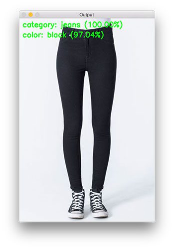
As expected, our network correctly classified the image as both “jeans” and “black”.
Let’s try a “red shirt”:
$ python classify.py --model fashion.model \
	--categorybin output/category_lb.pickle --colorbin output/color_lb.pickle \
	--image examples/red_shirt.jpg
Using TensorFlow backend.
[INFO] loading network...
[INFO] classifying image...
[INFO] category: shirt (100.00%)
[INFO] color: red (100.00%)
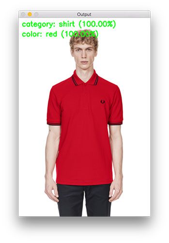
With 100% confidence for both class labels, our image definitely contains a “red shirt”. Remember, our network has seen other examples of “red shirts” during the training process.
Now let’s step back.
Take a look at our dataset and recall that it has never seen “red shoes” before, but it has seen “red” in the form of “dresses” and “shirts” as well as “shoes” with “black” color.
Is it possible to make the distinction that this unfamiliar test image contains “shoes” that are “red”?
Let’s find out:
$ python classify.py --model fashion.model \
	--categorybin output/category_lb.pickle --colorbin output/color_lb.pickle \
	--image examples/red_shoes.jpgUsing TensorFlow backend.
[INFO] loading network...
[INFO] classifying image...
[INFO] category: shoes (82.20%)
[INFO] color: red (99.99%)
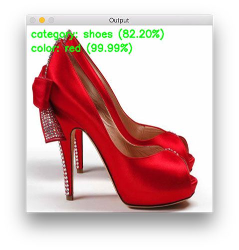
Bingo!
Looking at the results in the image, we were successful.
We’re off to a good start while presenting unfamiliar multi-output combinations. Our network design + training has paid off and we were able to recognize “red shoes” with high accuracy.
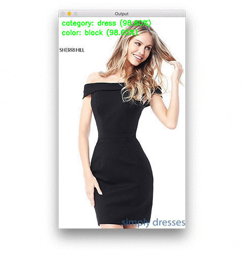
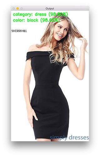
We’re not done yet — let’s present an image containing a “black dress” to our network. Remember, previously this same image did not yield a correct result in our multi-label classification tutorial.
I think we have a great chance at success this time around, so type the following command in your terminal:
$ python classify.py --model fashion.model \
	--categorybin output/category_lb.pickle --colorbin output/color_lb.pickle \
	--image examples/black_dress.jpg
Using TensorFlow backend.
[INFO] loading network...
[INFO] classifying image...
[INFO] category: dress (98.80%)
[INFO] color: black (98.65%)
Check out the class labels on the top-left of the image!
We achieved correct classification in both category and color with both reporting confidence of > 98% accuracy. We’ve accomplished our goal!
For sanity, let’s try one more unfamiliar combination: “blue shoes”. Enter the same command in your terminal, this time changing the --image argument to examples/blue_shoes.jpg :
$ python classify.py --model fashion.model \
	--categorybin output/category_lb.pickle --colorbin output/color_lb.pickle \
	--image examples/blue_shoes.jpg
Using TensorFlow backend.
[INFO] loading network...
[INFO] classifying image...
[INFO] category: shoes (100.00%)
[INFO] color: blue (99.05%)
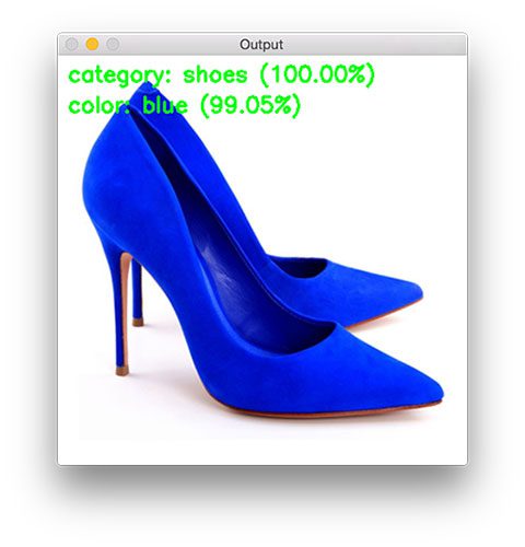
The same deal is confirmed — our network was not trained on “blue shoes” images but we were able to correctly classify them by using our two sub-networks along with multi-output and multi-loss classification.
What's next? I recommend PyImageSearch University.

30+ total classes • 39h 44m video • Last updated: 12/2021
★★★★★ 4.84 (128 Ratings) • 3,000+ Students Enrolled
I strongly believe that if you had the right teacher you could master computer vision and deep learning.
Do you think learning computer vision and deep learning has to be time-consuming, overwhelming, and complicated? Or has to involve complex mathematics and equations? Or requires a degree in computer science?
That’s not the case.
All you need to master computer vision and deep learning is for someone to explain things to you in simple, intuitive terms. And that’s exactly what I do. My mission is to change education and how complex Artificial Intelligence topics are taught.
If you're serious about learning computer vision, your next stop should be PyImageSearch University, the most comprehensive computer vision, deep learning, and OpenCV course online today. Here you’ll learn how to successfully and confidently apply computer vision to your work, research, and projects. Join me in computer vision mastery.
Inside PyImageSearch University you'll find:
- ✓ 30+ courses on essential computer vision, deep learning, and OpenCV topics
- ✓ 30+ Certificates of Completion
- ✓ 39h 44m on-demand video
- ✓ Brand new courses released every month, ensuring you can keep up with state-of-the-art techniques
- ✓ Pre-configured Jupyter Notebooks in Google Colab
- ✓ Run all code examples in your web browser — works on Windows, macOS, and Linux (no dev environment configuration required!)
- ✓ Access to centralized code repos for all 500+ tutorials on PyImageSearch
- ✓ Easy one-click downloads for code, datasets, pre-trained models, etc.
- ✓ Access on mobile, laptop, desktop, etc.
Summary
In today’s blog post, we learned how to utilize multiple outputs and multiple loss functions in the Keras deep learning library.
To accomplish this task, we defined a Keras architecture that is used for fashion/clothing classification called FashionNet.
The FashionNet architecture contains two forks:
- One fork is responsible for classifying the clothing type of a given input image (ex., shirt, dress, jeans, shoes, etc.).
- And the second fork is responsible for classifying the color of the clothing (black, red, blue, etc.).
This branch took place early in the network, essentially creating two “sub-networks” that are responsible for each of their respective classification tasks but both contained in the same network.
Most notably, multi-output classification enabled us to solve a nuisance from our previous post on multi-label classification where:
- We trained our network on six categories, including: black jeans, blue dresses, blue jeans, blue shirts, red dresses, and red shirts…
- …but we were unable to classify “black dress” as our network had never seen this combination of data before!
By creating two fully-connected heads and associated sub-networks (if necessary) we can train one head to classify clothing type and the other can learn how to recognize color — the end result is a network that can classify “black dress” even though it was never trained on such data!
Keep in mind though, you should always try to provide example training data for each class you want to recognize — deep neural networks, while powerful, are not “magic”!
You need to put in a best effort to train them properly and that includes gathering proper training data first.
I hope enjoyed today’s post on multi-output classification!
To be notified when future posts are published here on PyImageSearch, just enter your email address in the form below!

Download the Source Code and FREE 17-page Resource Guide
Enter your email address below to get a .zip of the code and a FREE 17-page Resource Guide on Computer Vision, OpenCV, and Deep Learning. Inside you'll find my hand-picked tutorials, books, courses, and libraries to help you master CV and DL!