Keras: Multiple Inputs and Mixed Data

Last updated on July 8, 2021.

In this tutorial, you will learn how to use Keras for multi-input and mixed data.

You will learn how to define a Keras architecture capable of accepting multiple inputs, including numerical, categorical, and image data. We’ll then train a single end-to-end network on this mixed data.

Today is the final installment in our three part series on Keras and regression:

1. Basic regression with Keras
2. Training a Keras CNN for regression prediction
3. Multiple inputs and mixed data with Keras (today’s post)

In this series of posts, we’ve explored regression prediction in the context of house price prediction.

The house price dataset we are using includes not only numerical and categorical data, but image data as well — we call multiple types of data mixed data as our model needs to be capable of accepting our multiple inputs (that are not of the same type) and computing a prediction on these inputs.

In the remainder of this tutorial you will learn how to:

1. Define a Keras model capable of accepting multiple inputs, including numerical, categorical, and image data, all at the same time.
2. Train an end-to-end Keras model on the mixed data inputs.
3. Evaluate our model using the multi-inputs.

To learn more about multiple inputs and mixed data with Keras, just keep reading!

• Update July 2021: Added section on the problems associated with one-hot encoding categorical data and how learning embeddings can help resolve the problem, especially when working in a multi-input network scenario.

Keras: Multiple Inputs and Mixed Data

2020-06-12 Update: This blog post is now TensorFlow 2+ compatible!

In the first part of this tutorial, we will briefly review the concept of both mixed data and how Keras can accept multiple inputs.

From there we’ll review our house prices dataset and the directory structure for this project.

Next, I’ll show you how to:

1. Load the numerical, categorical, and image data from disk.
2. Pre-process the data so we can train a network on it.
3. Prepare the mixed data so it can be applied to a multi-input Keras network.

Once our data has been prepared you’ll learn how to define and train a multi-input Keras model that accepts multiple types of input data in a single end-to-end network.

Finally, we’ll evaluate our multi-input and mixed data model on our testing set and compare the results to our previous posts in this series.

What is mixed data?

In machine learning, mixed data refers to the concept of having multiple types of independent data.

For example, let’s suppose we are machine learning engineers working at a hospital to develop a system capable of classifying the health of a patient.

We would have multiple types of input data for a given patient, including:

1. Numeric/continuous values, such as age, heart rate, blood pressure
2. Categorical values, including gender and ethnicity
3. Image data, such as any MRI, X-ray, etc.

All of these values constitute different data types; however, our machine learning model must be able to ingest this “mixed data” and make (accurate) predictions on it.

You will see the term “mixed data” in machine learning literature when working with multiple data modalities.

Developing machine learning systems capable of handling mixed data can be extremely challenging as each data type may require separate preprocessing steps, including scaling, normalization, and feature engineering.

Working with mixed data is still very much an open area of research and is often heavily dependent on the specific task/end goal.

We’ll be working with mixed data in today’s tutorial to help you get a feel for some of the challenges associated with it.

How can Keras accept multiple inputs?

Keras is able to handle multiple inputs (and even multiple outputs) via its functional API.

Learn more about 3 ways to create a Keras model with TensorFlow 2.0 (Sequential, Functional, and Model Subclassing).

The functional API, as opposed to the sequential API (which you almost certainly have used before via the Sequential class), can be used to define much more complex models that are non-sequential, including:

• Multi-input models
• Multi-output models
• Models that are both multiple input and multiple output
• Directed acyclic graphs
• Models with shared layers

For example, we may define a simple sequential neural network as:

model = Sequential()
model.add(Dense(8, input_shape=(10,), activation="relu"))
model.add(Dense(4, activation="relu"))
model.add(Dense(1, activation="linear"))

This network is a simple feedforward neural without with 10 inputs, a first hidden layer with 8 nodes, a second hidden layer with 4 nodes, and a final output layer used for regression.

We can define the sample neural network using the functional API:

inputs = Input(shape=(10,))
x = Dense(8, activation="relu")(inputs)
x = Dense(4, activation="relu")(x)
x = Dense(1, activation="linear")(x)
model = Model(inputs, x)

Notice how we are no longer relying on the Sequential class.

To see the power of Keras’ function API consider the following code where we create a model that accepts multiple inputs:

# define two sets of inputs
inputA = Input(shape=(32,))
inputB = Input(shape=(128,))

# the first branch operates on the first input
x = Dense(8, activation="relu")(inputA)
x = Dense(4, activation="relu")(x)
x = Model(inputs=inputA, outputs=x)

# the second branch opreates on the second input
y = Dense(64, activation="relu")(inputB)
y = Dense(32, activation="relu")(y)
y = Dense(4, activation="relu")(y)
y = Model(inputs=inputB, outputs=y)

# combine the output of the two branches
combined = concatenate([x.output, y.output])

# apply a FC layer and then a regression prediction on the
# combined outputs
z = Dense(2, activation="relu")(combined)
z = Dense(1, activation="linear")(z)

# our model will accept the inputs of the two branches and
# then output a single value
model = Model(inputs=[x.input, y.input], outputs=z)

Here you can see we are defining two inputs to our Keras neural network:

1. inputA : 32-dim
2. inputB : 128-dim

Lines 21-23 define a simple 32-8-4 network using Keras’ functional API.

Similarly, Lines 26-29 define a 128-64-32-4 network.

We then combine the outputs of both the x and y on Line 32. The outputs of x and y are both 4-dim so once we concatenate them we have a 8-dim vector.

We then apply two more fully-connected layers on Lines 36 and 37. The first layer has 2 nodes followed by a ReLU activation while the second layer has only a single node with a linear activation (i.e., our regression prediction).

The final step to building the multi-input model is to define a Model object which:

1. Accepts our two inputs
2. Defines the outputs as the final set of FC layers (i.e., z ).

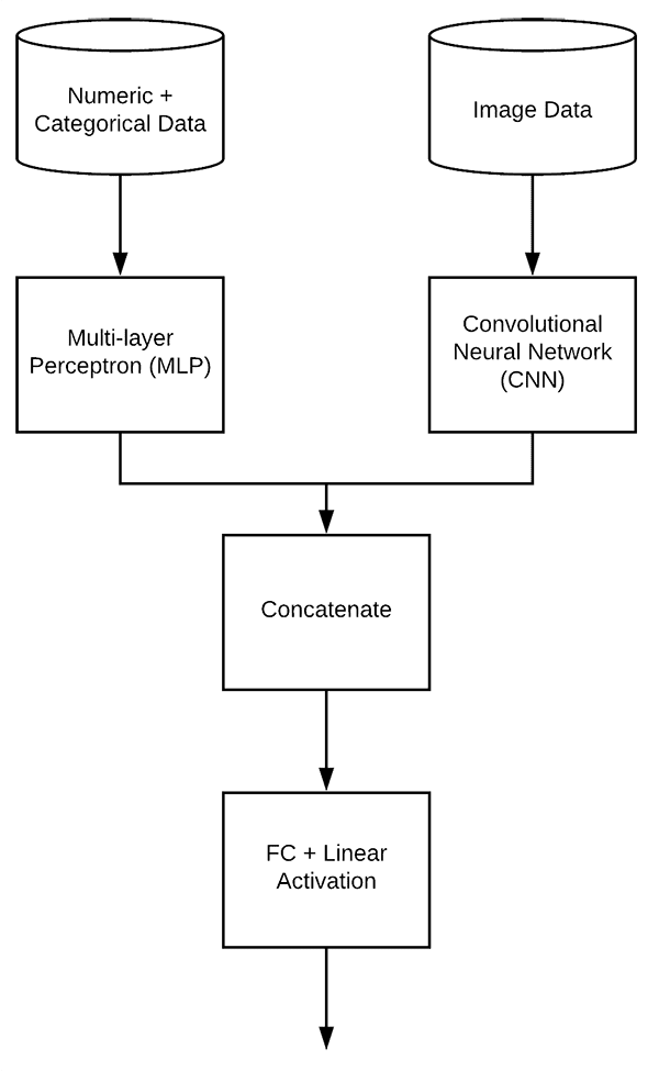
If you were to use Keras to visualize the model architecture it would look like the following:

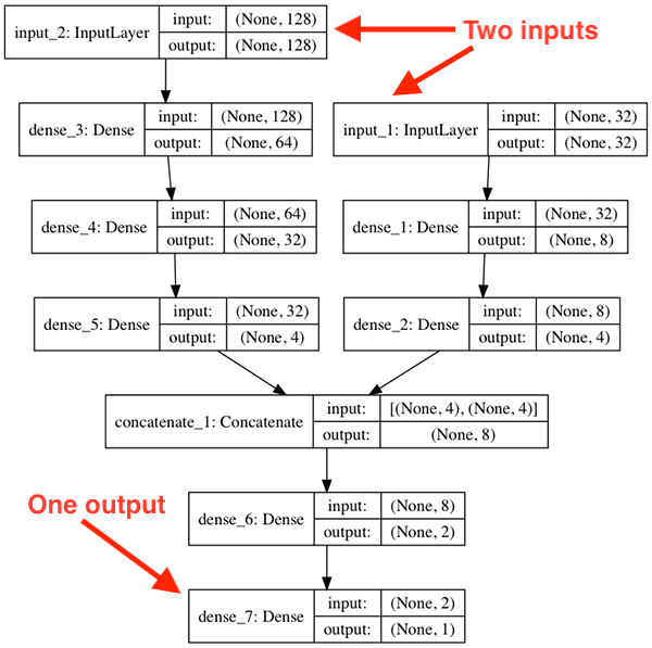
Notice how our model has two distinct branches.

The first branch accepts our 128-d input while the second branch accepts the 32-d input. These branches operate independently of each other until they are concatenated. From there a single value is output from the network.

In the remainder of this tutorial, you will learn how to create multiple input networks using Keras.

The House Prices dataset

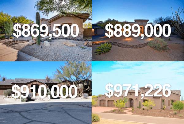
In this series of posts, we have been using the House Prices dataset from Ahmed and Moustafa’s 2016 paper, House price estimation from visual and textual features.

This dataset includes both numerical/categorical data along with images data for each of the 535 example houses in the dataset.

The numerical and categorical attributes include:

1. Number of bedrooms
2. Number of bathrooms
3. Area (i.e., square footage)
4. Zip code

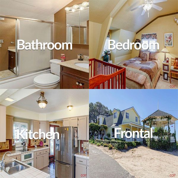
A total of four images are provided for each house as well:

1. Bedroom
2. Bathroom
3. Kitchen
4. Frontal view of the house

In the first post in this series, you learned how to train a Keras regression network on the numerical and categorical data.

Then, last week, you learned how to perform regression with a Keras CNN.

Today we are going to work with multiple inputs and mixed data with Keras.

We are going to accept both the numerical/categorical data along with our image data to the network.

Two branches of a network will be defined to handle each type of data. The branches will then be combined at the end to obtain our final house price prediction.

In this manner, we will be able to leverage Keras to handle both multiple inputs and mixed data.

Obtaining the House Prices dataset

To grab the source code for today’s post, use the “Downloads” section. Once you have the zip file, navigate to where you downloaded it, and extract it:

$ cd path/to/zip
$ unzip keras-multi-input.zip
$ cd keras-multi-input

And from there you can download the House Prices dataset via:

$ git clone https://github.com/emanhamed/Houses-dataset

The House Prices dataset should now be in the keras-multi-input directory which is the directory we are using for this project.

Configuring your development environment

To configure your system for this tutorial, I recommend following either of these tutorials:

• How to install TensorFlow 2.0 on Ubuntu
• How to install TensorFlow 2.0 on macOS

Either tutorial will help you configure you system with all the necessary software for this blog post in a convenient Python virtual environment.

Please note that PyImageSearch does not recommend or support Windows for CV/DL projects.

Project structure

Let’s take a look at how today’s project is organized:

$ tree --dirsfirst --filelimit 10
.
├── Houses-dataset
│   ├── Houses\ Dataset [2141 entries]
│   └── README.md
├── pyimagesearch
│   ├── __init__.py
│   ├── datasets.py
│   └── models.py
└── mixed_training.py

3 directories, 5 files

The Houses-dataset folder contains our House Prices dataset that we’re working with for this series. When we’re ready to run the mixed_training.py script, you’ll just need to provide a path as a command line argument to the dataset (I’ll show you exactly how this is done in the results section).

Today we’ll be reviewing three Python scripts:

• pyimagesearch/datasets.py : Handles loading and preprocessing our numerical/categorical data as well as our image data. We previously reviewed this script over the past two weeks, but I’ll be walking you through it again today.
• pyimagesearch/models.py : Contains our Multi-layer Perceptron (MLP) and Convolutional Neural Network (CNN). These components are the input branches to our multi-input, mixed data model. We reviewed this script last week and we’ll briefly review it today as well.
• mixed_training.py : Our training script will use the pyimagesearch module convenience functions to load + split the data and concatenate the two branches to our network + add the head. It will then train and evaluate the model.

Loading the numerical and categorical data

We covered how to load the numerical and categorical data for the house prices dataset in our Keras regression post but as a matter of completeness, we will review the code (in less detail) here today.

Be sure to refer to the previous post if you want a detailed walkthrough of the code.

Open up the datasets.py file and insert the following code:

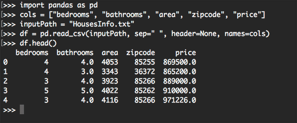
# import the necessary packages
from sklearn.preprocessing import LabelBinarizer
from sklearn.preprocessing import MinMaxScaler
import pandas as pd
import numpy as np
import glob
import cv2
import os

def load_house_attributes(inputPath):
	# initialize the list of column names in the CSV file and then
	# load it using Pandas
	cols = ["bedrooms", "bathrooms", "area", "zipcode", "price"]
	df = pd.read_csv(inputPath, sep=" ", header=None, names=cols)

	# determine (1) the unique zip codes and (2) the number of data
	# points with each zip code
	zipcodes = df["zipcode"].value_counts().keys().tolist()
	counts = df["zipcode"].value_counts().tolist()

	# loop over each of the unique zip codes and their corresponding
	# count
	for (zipcode, count) in zip(zipcodes, counts):
		# the zip code counts for our housing dataset is *extremely*
		# unbalanced (some only having 1 or 2 houses per zip code)
		# so let's sanitize our data by removing any houses with less
		# than 25 houses per zip code
		if count < 25:
			idxs = df[df["zipcode"] == zipcode].index
			df.drop(idxs, inplace=True)

	# return the data frame
	return df

Our imports are handled on Lines 2-8.

From there we define the load_house_attributes function on Lines 10-33. This function reads the numerical/categorical data from the House Prices dataset in the form of a CSV file via Pandas’ pd.read_csv on Lines 13 and 14.

The data is filtered to accommodate an imbalance. Some zipcodes only are represented by 1 or 2 houses, therefore we just go ahead and drop (Lines 23-30) any records where there are fewer than 25 houses from the zipcode. The result is a more accurate model later on.

Now let’s define the process_house_attributes function:

def process_house_attributes(df, train, test):
	# initialize the column names of the continuous data
	continuous = ["bedrooms", "bathrooms", "area"]

	# performin min-max scaling each continuous feature column to
	# the range [0, 1]
	cs = MinMaxScaler()
	trainContinuous = cs.fit_transform(train[continuous])
	testContinuous = cs.transform(test[continuous])

	# one-hot encode the zip code categorical data (by definition of
	# one-hot encoding, all output features are now in the range [0, 1])
	zipBinarizer = LabelBinarizer().fit(df["zipcode"])
	trainCategorical = zipBinarizer.transform(train["zipcode"])
	testCategorical = zipBinarizer.transform(test["zipcode"])

	# construct our training and testing data points by concatenating
	# the categorical features with the continuous features
	trainX = np.hstack([trainCategorical, trainContinuous])
	testX = np.hstack([testCategorical, testContinuous])

	# return the concatenated training and testing data
	return (trainX, testX)

This function applies min-max scaling to the continuous features via scikit-learn’s MinMaxScaler (Lines 41-43).

Then, one-hot encoding for the categorical features is computed, this time via scikit-learn’s LabelBinarizer (Lines 47-49).

The continuous and categorical features are then concatenated and returned (Lines 53-57).

Be sure to refer to the previous posts in this series for more details on the two functions we reviewed in this section:

1. Regression with Keras
2. Keras, Regression, and CNNs

Loading the image dataset

The next step is to define a helper function to load our input images. Again, open up the datasets.py file and insert the following code:

def load_house_images(df, inputPath):
	# initialize our images array (i.e., the house images themselves)
	images = []

	# loop over the indexes of the houses
	for i in df.index.values:
		# find the four images for the house and sort the file paths,
		# ensuring the four are always in the *same order*
		basePath = os.path.sep.join([inputPath, "{}_*".format(i + 1)])
		housePaths = sorted(list(glob.glob(basePath)))

The load_house_images function has three goals:

1. Load all photos from the House Prices dataset. Recall that we have four photos per house (Figure 6).
2. Generate a single montage image from the four photos. The montage will always be arranged as you see in the figure.
3. Append all of these home montages to a list/array and return to the calling function.

Beginning on Line 59, we define the function which accepts a Pandas dataframe and dataset inputPath .

From there, we proceed to:

• Initialize the images list (Line 61). We’ll be populating this list with all of the montage images that we build.
• Loop over houses in our data frame (Line 64). Inside the loop, we:
  • Grab the paths to the four photos for the current house (Lines 67 and 68).

Let’s keep making progress in the loop:

		# initialize our list of input images along with the output image
		# after *combining* the four input images
		inputImages = []
		outputImage = np.zeros((64, 64, 3), dtype="uint8")

		# loop over the input house paths
		for housePath in housePaths:
			# load the input image, resize it to be 32 32, and then
			# update the list of input images
			image = cv2.imread(housePath)
			image = cv2.resize(image, (32, 32))
			inputImages.append(image)

		# tile the four input images in the output image such the first
		# image goes in the top-right corner, the second image in the
		# top-left corner, the third image in the bottom-right corner,
		# and the final image in the bottom-left corner
		outputImage[0:32, 0:32] = inputImages[0]
		outputImage[0:32, 32:64] = inputImages[1]
		outputImage[32:64, 32:64] = inputImages[2]
		outputImage[32:64, 0:32] = inputImages[3]

		# add the tiled image to our set of images the network will be
		# trained on
		images.append(outputImage)

	# return our set of images
	return np.array(images)

The code so far has accomplished the first goal discussed above (grabbing the four house images per house). Let’s wrap up the load_house_images function:

• Still inside the loop, we:
  • Perform initializations (Lines 72 and 73). Our inputImages will be in list form containing four photos of each record. Our outputImage will be the montage of the photos (like Figure 6).
  • Loop over 4 photos (Line 76):
    • Load, resize, and append each photo to inputImages (Lines 79-81).
  • Create the tiling (a montage) for the four house images (Lines 87-90) with:
    • The bathroom image in the top-left.
    • The bedroom image in the top-right.
    • The frontal view in the bottom-right.
    • The kitchen in the bottom-left.
  • Append the tiling/montage outputImage to images (Line 94).
• Jumping out of the loop, we return all the images in the form of a NumPy array (Line 97).

We’ll have as many images as there are records we’re training with (remember, we dropped a few of them in the process_house_attributes function).

Each of our tiled images will look like Figure 6 (without the overlaid text of course). You can see the four photos therein have been arranged in a montage (I’ve used larger image dimensions so we can better visualize what the code is doing). Just as our numerical and categorical attributes represent the house, these four photos (tiled into a single image) will represent the visual aesthetics of the house.

If you need to review this process in further detail, be sure to refer to last week’s post.

Defining our Multi-layer Perceptron (MLP) and Convolutional Neural Network (CNN)

As you’ve gathered thus far, we’ve had to massage our data carefully using multiple libraries: Pandas, scikit-learn, OpenCV, and NumPy.

We’ve organized and pre-processed the two modalities of our dataset at this point via datasets.py :

• Numeric and categorical data
• Image data

The skills we’ve used in order to accomplish this have been developed through experience + practice, machine learning best practices, and behind the scenes of this blog post, a little bit of debugging. Please don’t overlook what we’ve discussed so far using our data massaging skills as it is key to the rest of our project’s success.

Let’s shift gears and discuss our multi-input and mixed data network that we’ll build with Keras’ functional API.

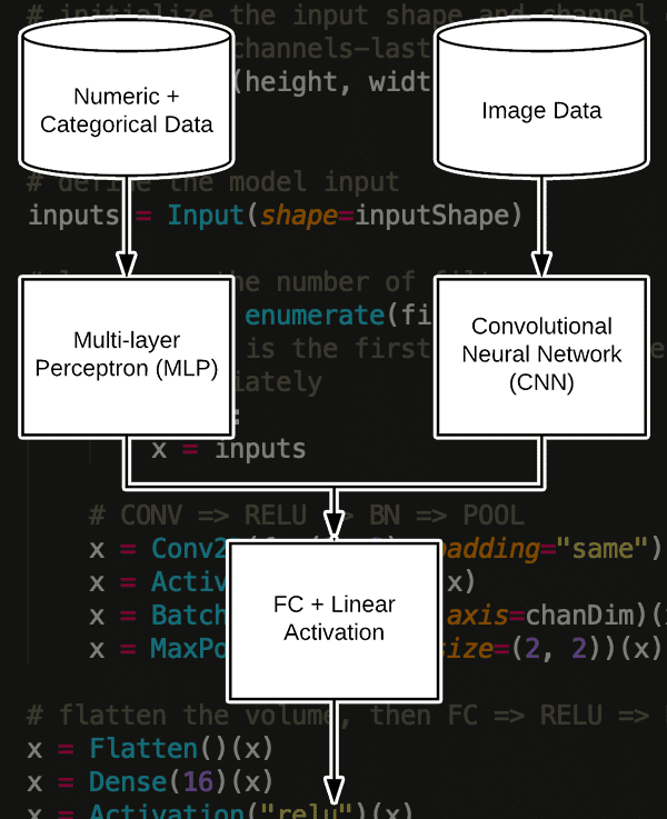
In order to build our multi-input network we will need two branches:

• The first branch will be a simple Multi-layer Perceptron (MLP) designed to handle the categorical/numerical inputs.
• The second branch will be a Convolutional Neural Network to operate over the image data.
• These branches will then be concatenated together to form the final multi-input Keras model.

We’ll handle building the final concatenated multi-input model in the next section — our current task is to define the two branches.

Open up the models.py file and insert the following code:

# import the necessary packages
from tensorflow.keras.models import Sequential
from tensorflow.keras.layers import BatchNormalization
from tensorflow.keras.layers import Conv2D
from tensorflow.keras.layers import MaxPooling2D
from tensorflow.keras.layers import Activation
from tensorflow.keras.layers import Dropout
from tensorflow.keras.layers import Dense
from tensorflow.keras.layers import Flatten
from tensorflow.keras.layers import Input
from tensorflow.keras.models import Model

def create_mlp(dim, regress=False):
	# define our MLP network
	model = Sequential()
	model.add(Dense(8, input_dim=dim, activation="relu"))
	model.add(Dense(4, activation="relu"))

	# check to see if the regression node should be added
	if regress:
		model.add(Dense(1, activation="linear"))

	# return our model
	return model

Lines 2-11 handle our Keras imports. You’ll see each of the imported functions/classes going forward in this script.

Our categorical/numerical data will be processed by a simple Multi-layer Perceptron (MLP).

The MLP is defined by create_mlp on Lines 13-24.

Discussed in detail in the first post in this series, the MLP relies on the Keras Sequential API. Our MLP is quite simple having:

• A fully connected (Dense ) input layer with ReLU activation (Line 16).
• A fully-connected hidden layer, also with ReLU activation (Line 17).
• And finally, an optional regression output with linear activation (Lines 20 and 21).

While we used the regression output of the MLP in the first post, it will not be used in this multi-input, mixed data network. As you’ll soon see, we’ll be setting regress=False explicitly even though it is the default as well. Regression will actually be performed later on the head of the entire multi-input, mixed data network (the bottom of Figure 7).

The MLP branch is returned on Line 24.

Referring back to Figure 7, we’ve now built the top-left branch of our network.

Let’s now define the top-right branch of our network, a CNN:

def create_cnn(width, height, depth, filters=(16, 32, 64), regress=False):
	# initialize the input shape and channel dimension, assuming
	# TensorFlow/channels-last ordering
	inputShape = (height, width, depth)
	chanDim = -1

	# define the model input
	inputs = Input(shape=inputShape)

	# loop over the number of filters
	for (i, f) in enumerate(filters):
		# if this is the first CONV layer then set the input
		# appropriately
		if i == 0:
			x = inputs

		# CONV => RELU => BN => POOL
		x = Conv2D(f, (3, 3), padding="same")(x)
		x = Activation("relu")(x)
		x = BatchNormalization(axis=chanDim)(x)
		x = MaxPooling2D(pool_size=(2, 2))(x)

The create_cnn function handles the image data and accepts five parameters:

• width : The width of the input images in pixels.
• height : How many pixels tall the input images are.
• depth : The number of channels in our input images. For RGB color images, it is three.
• filters : A tuple of progressively larger filters so that our network can learn more discriminate features.
• regress : A boolean indicating whether or not a fully-connected linear activation layer will be appended to the CNN for regression purposes.

The inputShape of our network is defined on Line 29. It assumes “channels last” ordering for the TensorFlow backend.

The Input to the model is defined via the inputShape on (Line 33).

From there we begin looping over the filters and create a set of CONV => RELU > BN => POOL layers. Each iteration of the loop appends these layers. Be sure to check out Chapter 11 from the Starter Bundle of Deep Learning for Computer Vision with Python for more information on these layer types if you are unfamiliar.

Let’s finish building the CNN branch of our network:

	# flatten the volume, then FC => RELU => BN => DROPOUT
	x = Flatten()(x)
	x = Dense(16)(x)
	x = Activation("relu")(x)
	x = BatchNormalization(axis=chanDim)(x)
	x = Dropout(0.5)(x)

	# apply another FC layer, this one to match the number of nodes
	# coming out of the MLP
	x = Dense(4)(x)
	x = Activation("relu")(x)

	# check to see if the regression node should be added
	if regress:
		x = Dense(1, activation="linear")(x)

	# construct the CNN
	model = Model(inputs, x)

	# return the CNN
	return model

We Flatten the next layer (Line 49) and then add a fully-connected layer with BatchNormalization and Dropout (Lines 50-53).

Another fully-connected layer is applied to match the four nodes coming out of the multi-layer perceptron (Lines 57 and 58). Matching the number of nodes is not a requirement but it does help balance the branches.

On Lines 61 and 62, a check is made to see if the regression node should be appended; it is then added in accordingly. Again, we will not be conducting regression at the end of this branch either. Regression will be performed on the head of the multi-input, mixed data network (the very bottom of Figure 7).

Finally, the model is constructed from our inputs and all the layers we’ve assembled together, x (Line 65).

We can then return the CNN branch to the calling function (Line 68).

Now that we’ve defined both branches of the multi-input Keras model, let’s learn how we can combine them!

Multiple inputs with Keras

We are now ready to build our final Keras model capable of handling both multiple inputs and mixed data. This is where the branches come together and ultimately where the “magic” happens. Training will also happen in this script.

Create a new file named mixed_training.py , open it up, and insert the following code:

# import the necessary packages
from pyimagesearch import datasets
from pyimagesearch import models
from sklearn.model_selection import train_test_split
from tensorflow.keras.layers import Dense
from tensorflow.keras.models import Model
from tensorflow.keras.optimizers import Adam
from tensorflow.keras.layers import concatenate
import numpy as np
import argparse
import locale
import os

# construct the argument parser and parse the arguments
ap = argparse.ArgumentParser()
ap.add_argument("-d", "--dataset", type=str, required=True,
	help="path to input dataset of house images")
args = vars(ap.parse_args())

Our imports and command line arguments are handled first.

Notable imports include:

• datasets : Our three convenience functions for loading/processing the CSV data and loading/pre-processing the house photos from the Houses Dataset.
• models : Our MLP and CNN input branches which will serve as our multi-input, mixed data.
• train_test_split : A scikit-learn function to construct our training/testing data splits.
• concatenate : A special Keras function which will accept multiple inputs.
• argparse : Handles parsing command line arguments.

We have one command line argument to parse on Lines 15-18, --dataset , which is the path to where you downloaded the House Prices dataset.

Let’s load our numerical/categorical data and image data:

# construct the path to the input .txt file that contains information
# on each house in the dataset and then load the dataset
print("[INFO] loading house attributes...")
inputPath = os.path.sep.join([args["dataset"], "HousesInfo.txt"])
df = datasets.load_house_attributes(inputPath)

# load the house images and then scale the pixel intensities to the
# range [0, 1]
print("[INFO] loading house images...")
images = datasets.load_house_images(df, args["dataset"])
images = images / 255.0

Here we’ve loaded the House Prices dataset as a Pandas dataframe (Lines 23 and 24).

Then we’ve loaded our images and scaled them to the range [0, 1] (Lines 29-30).

Be sure to review the load_house_attributes and load_house_images functions above if you need a reminder on what these functions are doing under the hood.

Now that our data is loaded, we’re going to construct our training/testing splits, scale the prices, and process the house attributes:

# partition the data into training and testing splits using 75% of
# the data for training and the remaining 25% for testing
print("[INFO] processing data...")
split = train_test_split(df, images, test_size=0.25, random_state=42)
(trainAttrX, testAttrX, trainImagesX, testImagesX) = split

# find the largest house price in the training set and use it to
# scale our house prices to the range [0, 1] (will lead to better
# training and convergence)
maxPrice = trainAttrX["price"].max()
trainY = trainAttrX["price"] / maxPrice
testY = testAttrX["price"] / maxPrice

# process the house attributes data by performing min-max scaling
# on continuous features, one-hot encoding on categorical features,
# and then finally concatenating them together
(trainAttrX, testAttrX) = datasets.process_house_attributes(df,
	trainAttrX, testAttrX)

Our training and testing splits are constructed on Lines 35 and 36. We’ve allocated 75% of our data for training and 25% of our data for testing.

From there, we find the maxPrice from the training set (Line 41) and scale the training and testing data accordingly (Lines 42 and 43). Having the pricing data in the range [0, 1] leads to better training and convergence.

Finally, we go ahead and process our house attributes by performing min-max scaling on continuous features and one-hot encoding on categorical features. The process_house_attributes function handles these actions and concatenates the continuous and categorical features together, returning the results (Lines 48 and 49).

Ready for some magic?

Okay, I lied. There isn’t actually any “magic” going on in this next code block! But we will concatenate the branches of our network and finish our multi-input Keras network:

# create the MLP and CNN models
mlp = models.create_mlp(trainAttrX.shape[1], regress=False)
cnn = models.create_cnn(64, 64, 3, regress=False)

# create the input to our final set of layers as the *output* of both
# the MLP and CNN
combinedInput = concatenate([mlp.output, cnn.output])

# our final FC layer head will have two dense layers, the final one
# being our regression head
x = Dense(4, activation="relu")(combinedInput)
x = Dense(1, activation="linear")(x)

# our final model will accept categorical/numerical data on the MLP
# input and images on the CNN input, outputting a single value (the
# predicted price of the house)
model = Model(inputs=[mlp.input, cnn.input], outputs=x)

Handling multiple inputs with Keras is quite easy when you’ve organized your code and models.

On Lines 52 and 53, we create our mlp and cnn models. Notice that regress=False — our regression head comes later on Line 62.

We’ll then concatenate the mlp.output and cnn.output as shown on Line 57. I’m calling this our combinedInput because it is the input to the rest of the network (from Figure 3 this is concatenate_1 where the two branches come together).

The combinedInput to the final layers in the network is based on the output of both the MLP and CNN branches’ 8-4-1 FC layers (since each of the 2 branches outputs a 4-dim FC layer and then we concatenate them to create an 8-dim vector).

We tack on a fully connected layer with four neurons to the combinedInput (Line 61).

Then we add our "linear" activation regression head (Line 62), the output of which is the predicted price.

Our Model is defined using the inputs of both branches as our multi-input and the final set of layers x as the output (Line 67).

Let’s go ahead and compile, train, and evaluate our newly formed model :

# compile the model using mean absolute percentage error as our loss,
# implying that we seek to minimize the absolute percentage difference
# between our price *predictions* and the *actual prices*
opt = Adam(lr=1e-3, decay=1e-3 / 200)
model.compile(loss="mean_absolute_percentage_error", optimizer=opt)

# train the model
print("[INFO] training model...")
model.fit(
	x=[trainAttrX, trainImagesX], y=trainY,
	validation_data=([testAttrX, testImagesX], testY),
	epochs=200, batch_size=8)

# make predictions on the testing data
print("[INFO] predicting house prices...")
preds = model.predict([testAttrX, testImagesX])

Our model is compiled with "mean_absolute_percentage_error" loss and an Adam optimizer with learning rate decay (Lines 72 and 73).

Training is kicked off on Lines 77-80. This is known as fitting the model (and is also where all the weights are tuned by the process known as backpropagation).

Calling model.predict on our testing data (Line 84) allows us to grab predictions for evaluating our model. Let’s perform evaluation now:

# compute the difference between the *predicted* house prices and the
# *actual* house prices, then compute the percentage difference and
# the absolute percentage difference
diff = preds.flatten() - testY
percentDiff = (diff / testY) * 100
absPercentDiff = np.abs(percentDiff)

# compute the mean and standard deviation of the absolute percentage
# difference
mean = np.mean(absPercentDiff)
std = np.std(absPercentDiff)

# finally, show some statistics on our model
locale.setlocale(locale.LC_ALL, "en_US.UTF-8")
print("[INFO] avg. house price: {}, std house price: {}".format(
	locale.currency(df["price"].mean(), grouping=True),
	locale.currency(df["price"].std(), grouping=True)))
print("[INFO] mean: {:.2f}%, std: {:.2f}%".format(mean, std))

To evaluate our model, we have computed absolute percentage difference (Lines 89-91) and used it to derive our final metrics (Lines 95 and 96).

These metrics (price mean, price standard deviation, and mean + standard deviation of the absolute percentage difference) are printed to the terminal with proper currency locale formatting (Lines 100-103).

Multi-input and mixed data results

Finally, we are ready to train our multi-input network on our mixed data!

Make sure you have:

1. Configured your dev environment according to the first tutorial in this series.
2. Used the “Downloads” section of this tutorial to download the source code.
3. Downloaded the house prices dataset using the instructions in the “Obtaining the House Prices dataset” section above.

From there, open up a terminal and execute the following command to kick off training the network:

$ python mixed_training.py --dataset Houses-dataset/Houses\ Dataset/
[INFO] loading house attributes...
[INFO] loading house images...
[INFO] processing data...
[INFO] training model...
Epoch 1/200
34/34 [==============================] - 0s 10ms/step - loss: 972.0082 - val_loss: 137.5819
Epoch 2/200
34/34 [==============================] - 0s 4ms/step - loss: 708.1639 - val_loss: 873.5765
Epoch 3/200
34/34 [==============================] - 0s 5ms/step - loss: 551.8876 - val_loss: 1078.9347
Epoch 4/200
34/34 [==============================] - 0s 3ms/step - loss: 347.1892 - val_loss: 888.7679
Epoch 5/200
34/34 [==============================] - 0s 4ms/step - loss: 258.7427 - val_loss: 986.9370
Epoch 6/200
34/34 [==============================] - 0s 3ms/step - loss: 217.5041 - val_loss: 665.0192
Epoch 7/200
34/34 [==============================] - 0s 3ms/step - loss: 175.1175 - val_loss: 435.5834
Epoch 8/200
34/34 [==============================] - 0s 5ms/step - loss: 156.7351 - val_loss: 465.2547
Epoch 9/200
34/34 [==============================] - 0s 4ms/step - loss: 133.5550 - val_loss: 718.9653
Epoch 10/200
34/34 [==============================] - 0s 3ms/step - loss: 115.4481 - val_loss: 880.0882
...
Epoch 191/200
34/34 [==============================] - 0s 4ms/step - loss: 23.4761 - val_loss: 23.4792
Epoch 192/200
34/34 [==============================] - 0s 5ms/step - loss: 21.5748 - val_loss: 22.8284
Epoch 193/200
34/34 [==============================] - 0s 3ms/step - loss: 21.7873 - val_loss: 23.2362
Epoch 194/200
34/34 [==============================] - 0s 6ms/step - loss: 22.2006 - val_loss: 24.4601
Epoch 195/200
34/34 [==============================] - 0s 3ms/step - loss: 22.1863 - val_loss: 23.8873
Epoch 196/200
34/34 [==============================] - 0s 4ms/step - loss: 23.6857 - val_loss: 1149.7415
Epoch 197/200
34/34 [==============================] - 0s 4ms/step - loss: 23.0267 - val_loss: 86.4044
Epoch 198/200
34/34 [==============================] - 0s 4ms/step - loss: 22.7724 - val_loss: 29.4979
Epoch 199/200
34/34 [==============================] - 0s 3ms/step - loss: 23.1597 - val_loss: 23.2382
Epoch 200/200
34/34 [==============================] - 0s 3ms/step - loss: 21.9746 - val_loss: 27.5241
[INFO] predicting house prices...
[INFO] avg. house price: $533,388.27, std house price: $493,403.08
[INFO] mean: 27.52%, std: 22.19%

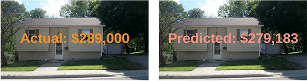
Our mean absolute percentage error starts off very high but continues to fall throughout the training process.

By the end of training, we are obtaining of 27.52% mean absolute percentage error on our testing set, implying that, on average, our network will be ~26-27% off in its house price predictions.

Let’s compare this result to our previous two posts in the series:

1. Using just an MLP on the numerical/categorical data: 22.71%
2. Using just a CNN on the image data: 56.91%

As you can see, working with mixed data by:

1. Combining our numerical/categorical data along with image data
2. And training a multi-input model on the mixed data…

…has led to a model that performs well, but not even as great as the simpler MLP method!

Note: If you run the experiment enough times, you may achieve results as good as [INFO] mean: 19.79%, std: 17.93% due to the stochastic nature of weight initialization.

Using embeddings to improve model architecture and accuracy

Before we could even train our multi-input network, we first needed to preprocess our data, including:

1. Applying min-max scaling to our continuous features
2. Applying one-hot encoding to our categorical features

However, there are two primary issues one-hot encoding our categorical values:

1. High dimensionality: If there are many unique categories then the output transformed one-hot encoded vector can become unmanageable.
2. No concept of “similar” categories: After applying one-hot encoding there is no guarantee that “similar” categories are placed closer together in the N–dimensional space than non-similar ones.

For example, let’s say we are trying to encode categories of fruits, including:

1. Granny Smith apples
2. Honeycrisp apples
3. Bananas

Intuition tells us that in an N-dimensional space the Granny Smith apples and Honeycrisp apples should live closer together than the bananas; however, one-hot encoding makes no such guarantee!

Luckily, we can overcome this problem by learning “embeddings” using our neural network. Don’t get me wrong, learning embeddings is much harder than simply using one-hot encodings; however, the accuracy of the model can jump significantly, and you won’t have to deal with the two issues mentioned above.

Here are some resources to help you get started with embeddings and deep learning:

• Google Developers guide
• Understanding Embedding Layer in Keras
• Deep Learning for Tabular Data using PyTorch

Summary

In this tutorial, you learned how to define a Keras network capable of accepting multiple inputs.

You learned how to work with mixed data using Keras as well.

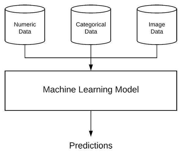
To accomplish these goals we defined a multiple input neural network capable of accepting:

• Numerical data
• Categorical data
• Image data

The numerical data was min-max scaled to the range [0, 1] prior to training. Our categorical data was one-hot encoded (also ensuring the resulting integer vectors were in the range [0, 1]).

The numerical and categorical data were then concatenated into a single feature vector to form the first input to the Keras network.

Our image data was also scaled to the range [0, 1] — this data served as the second input to the Keras network.

One branch of the model included strictly fully-connected layers (for the concatenated numerical and categorical data) while the second branch of the multi-input model was essentially a small Convolutional Neural Network.

The outputs of both branches were combined and a single output (the regression prediction) was defined.

In this manner, we were able to train our multiple input network end-to-end, resulting in accuracy almost as good as just one of the inputs alone.

I hope you enjoyed today’s blog post — if you ever need to work with multiple inputs and mixed data in your own projects definitely consider using the code covered in this tutorial as a template.

From there you can modify the code to your own needs.

To download the source code, and be notified when future tutorials are published here on PyImageSearch, just enter your email address in the form below!