Grad-CAM: Visualize class activation maps with Keras, TensorFlow, and Deep Learning

In this tutorial, you will learn how to visualize class activation maps for debugging deep neural networks using an algorithm called Grad-CAM. We’ll then implement Grad-CAM using Keras and TensorFlow.

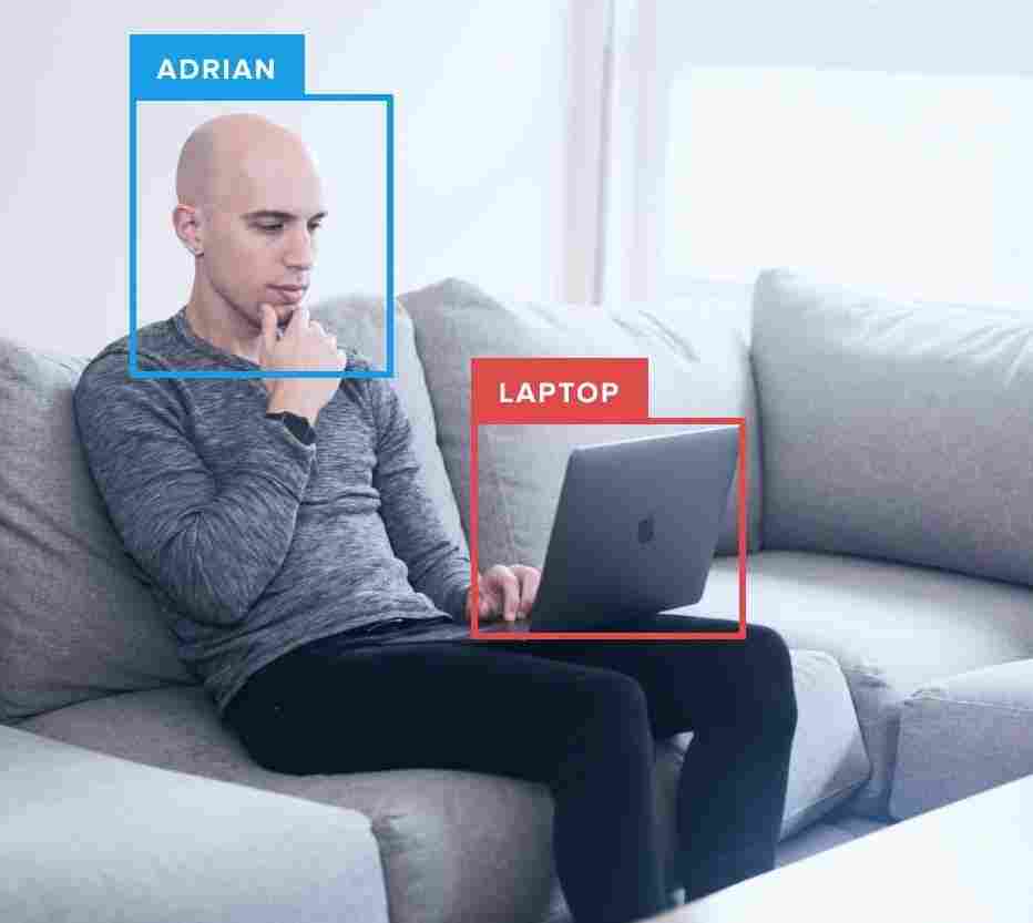
While deep learning has facilitated unprecedented accuracy in image classification, object detection, and image segmentation, one of their biggest problems is model interpretability, a core component in model understanding and model debugging.

In practice, deep learning models are treated as “black box” methods, and many times we have no reasonable idea as to:

• Where the network is “looking” in the input image
• Which series of neurons activated in the forward-pass during inference/prediction
• How the network arrived at its final output

That raises an interesting question — how can you trust the decisions of a model if you cannot properly validate how it arrived there?

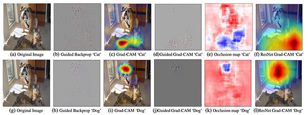
To help deep learning practitioners visually debug their models and properly understand where it’s “looking” in an image, Selvaraju et al. created Gradient-weighted Class Activation Mapping, or more simply, Grad-CAM:

Grad-CAM uses the gradients of any target concept (say logits for “dog” or even a caption), flowing into the final convolutional layer to produce a coarse localization map highlighting the important regions in the image for predicting the concept.”

Using Grad-CAM, we can visually validate where our network is looking, verifying that it is indeed looking at the correct patterns in the image and activating around those patterns.

If the network is not activating around the proper patterns/objects in the image, then we know:

• Our network hasn’t properly learned the underlying patterns in our dataset
• Our training procedure needs to be revisited
• We may need to collect additional data
• And most importantly, our model is not ready for deployment.

Grad-CAM is a tool that should be in any deep learning practitioner’s toolbox — take the time to learn how to apply it now.

To learn how to use Grad-CAM to debug your deep neural networks and visualize class activation maps with Keras and TensorFlow, just keep reading!

Grad-CAM: Visualize class activation maps with Keras, TensorFlow, and Deep Learning

In the first part of this article, I’ll share with you a cautionary tale on the importance of debugging and visually verifying that your convolutional neural network is “looking” at the right places in an image.

From there, we’ll dive into Grad-CAM, an algorithm that can be used visualize the class activation maps of a Convolutional Neural Network (CNN), thereby allowing you to verify that your network is “looking” and “activating” at the correct locations.

We’ll then implement Grad-CAM using Keras and TensorFlow.

After our Grad-CAM implementation is complete, we’ll look at a few examples of visualizing class activation maps.

Why would we want to visualize class activation maps in Convolutional Neural Networks?

There’s an old urban legend in the computer vision community that researchers use to caution budding machine learning practitioners against the dangers of deploying a model without first verifying that it’s working properly.

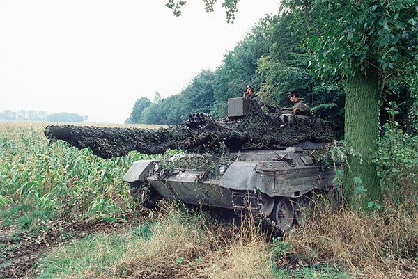
In this tale, the United States Army wanted to use neural networks to automatically detect camouflaged tanks.

Researchers assigned to the project gathered a dataset of 200 images:

• 100 of which contained camouflaged tanks hiding in trees
• 100 of which did not contain tanks and were images solely of trees/forest

The researchers took this dataset and then split it into an even 50/50 training and testing split, ensuring the class labels were balanced.

A neural network was trained on the training set and obtained a 100% accuracy. The researchers were incredibly pleased with this result and eagerly applied it to to their testing data. Once again, they obtained 100% accuracy.

The researchers called the Pentagon, excited with the news that they had just “solved” camouflaged tank detection.

A few weeks later, the research team received a call from the Pentagon — they were extremely unhappy with the performance of the camouflaged tank detector. The neural network that performed so well in the lab was performing terribly in the field.

Flummoxed, the researchers returned to their experiments, training model after model using different training procedures, only to arrive at the same result — 100% accuracy on both their training and testing sets.

It wasn’t until one clever researcher visually inspected their dataset and finally realized the problem:

• Photos of camouflaged tanks were captured on sunny days
• Images of the forest (without tanks) were captured on cloudy days

Essentially, the U.S. Army had created a multimillion dollar cloud detector.

While not true, this old urban legend does a good job illustrating the importance of model interoperability.

Had the research team had an algorithm like Grad-CAM, they would have noticed that the model was activating around the presence/absence of clouds, and not the tanks themselves (hence their problem).

Grad-CAM would have saved taxpayers millions of dollars, and not to mention, allowed the researchers to save face with the Pentagon — after a catastrophe like that, it’s unlikely they would be getting any more work or research grants.

What is Gradient-weighted Class Activation Mapping (Grad-CAM) and why would we use it?

As a deep learning practitioner, it’s your responsibility to ensure your model is performing correctly. One way you can do that is to debug your model and visually validate that it is “looking” and “activating” at the correct locations in an image.

To help deep learning practitioners debug their networks, Selvaraju et al. published a novel paper entitled, Grad-CAM: Visual Explanations from Deep Networks via Gradient-based Localization.

This method is:

• Easily implemented
• Works with nearly any Convolutional Neural Network architecture
• Can be used to visually debug where a network is looking in an image

Grad-CAM works by (1) finding the final convolutional layer in the network and then (2) examining the gradient information flowing into that layer.

The output of Grad-CAM is a heatmap visualization for a given class label (either the top, predicted label or an arbitrary label we select for debugging). We can use this heatmap to visually verify where in the image the CNN is looking.

For more information on how Grad-CAM works, I would recommend you read Selvaraju et al.’s paper as well as this excellent article by Divyanshu Mishra (just note that their implementation will not work with TensorFlow 2.0 while ours does work with TF 2.0).

Configuring your development environment

In order to use our Grad-CAM implementation, we need to configure our system with a few software packages including:

• TensorFlow (2.0 recommended)
• OpenCV
• imutils

Luckily, each of these packages is pip-installable. My personal recommendation is for you to follow one of my TensorFlow 2.0 installation tutorials:

• How to install TensorFlow 2.0 on Ubuntu (Ubuntu 18.04 OS; CPU and optional NVIDIA GPU)
• How to install TensorFlow 2.0 on macOS (Catalina and Mojave OSes)

Please note: PyImageSearch does not support Windows — refer to our FAQ. While we do not support Windows, the code presented in this blog post will work on Windows with a properly configured system.

Either of those tutorials will teach you how to configure a Python virtual environment with all the necessary software for this tutorial. I highly encourage virtual environments for Python work — industry considers them a best practice as well. If you’ve never worked with a Python virtual environment, you can learn more about them in this RealPython article.

Once your system is configured, you are ready to follow the rest of this tutorial.

Project structure

Let’s inspect our tutorial’s project structure. But first, be sure to grab the code and example images from the “Downloads” section of this blog post. From there, extract the files, and use the tree command in your terminal:

$ tree --dirsfirst
.
├── images
│   ├── beagle.jpg
│   ├── soccer_ball.jpg
│   └── space_shuttle.jpg
├── pyimagesearch
│   ├── __init__.py
│   └── gradcam.py
└── apply_gradcam.py

2 directories, 6 files

The pyimagesearch module today contains the Grad-CAM implementation inside the GradCAM class.

Our apply_gradcam.py driver script accepts any of our sample images/ and applies either a VGG16 or ResNet CNN trained on ImageNet to both (1) compute the Grad-CAM heatmap and (2) display the results in an OpenCV window.

Let’s dive into the implementation.

Implementing Grad-CAM using Keras and TensorFlow

Despite the fact that the Grad-CAM algorithm is relatively straightforward, I struggled to find a TensorFlow 2.0-compatible implementation.

The closest one I found was in tf-explain; however, that method could only be used when training — it could not be used after a model had been trained.

Therefore, I decided to create my own Grad-CAM implementation, basing my work on that of tf-explain, ensuring that my Grad-CAM implementation:

• Is compatible with Keras and TensorFlow 2.0
• Could be used after a model was already trained
• And could also be easily modified to work as a callback during training (not covered in this post)

Let’s dive into our Keras and TensorFlow Grad-CAM implementation.

Open up the gradcam.py file in your project directory structure, and let’s get started:

# import the necessary packages
from tensorflow.keras.models import Model
import tensorflow as tf
import numpy as np
import cv2

class GradCAM:
	def __init__(self, model, classIdx, layerName=None):
		# store the model, the class index used to measure the class
		# activation map, and the layer to be used when visualizing
		# the class activation map
		self.model = model
		self.classIdx = classIdx
		self.layerName = layerName

		# if the layer name is None, attempt to automatically find
		# the target output layer
		if self.layerName is None:
			self.layerName = self.find_target_layer()

Before we define the GradCAM class, we need to import several packages. These include a TensorFlow Model for which we will construct our gradient model, NumPy for mathematical calculations, and OpenCV.

Our GradCAM class and constructor are then defined beginning on Lines 7 and 8. The constructor accepts and stores:

• A TensorFlow model which we’ll use to compute a heatmap
• The classIdx — a specific class index that we’ll use to measure our class activation heatmap
• An optional CONV layerName of the model in case we want to visualize the heatmap of a specific layer of our CNN; otherwise, if a specific layer name is not provided, we will automatically infer on the final CONV/POOL layer of the model architecture (Lines 18 and 19)

Now that our constructor is defined and our class attributes are set, let’s define a method to find our target layer:

	def find_target_layer(self):
		# attempt to find the final convolutional layer in the network
		# by looping over the layers of the network in reverse order
		for layer in reversed(self.model.layers):
			# check to see if the layer has a 4D output
			if len(layer.output_shape) == 4:
				return layer.name

		# otherwise, we could not find a 4D layer so the GradCAM
		# algorithm cannot be applied
		raise ValueError("Could not find 4D layer. Cannot apply GradCAM.")

Our find_target_layer function loops over all layers in the network in reverse order, during which time it checks to see if the current layer has a 4D output (implying a CONV or POOL layer).

If find such a 4D output, we return that layer name (Lines 24-27).

Otherwise, if the network does not have a 4D output, then we cannot apply Grad-CAM, at which point, we raise a ValueError exception, causing our program to stop (Line 31).

In our next function, we’ll compute our visualization heatmap, given an input image:

	def compute_heatmap(self, image, eps=1e-8):
		# construct our gradient model by supplying (1) the inputs
		# to our pre-trained model, (2) the output of the (presumably)
		# final 4D layer in the network, and (3) the output of the
		# softmax activations from the model
		gradModel = Model(
			inputs=[self.model.inputs],
			outputs=[self.model.get_layer(self.layerName).output,
				self.model.output])

Line 33 defines the compute_heatmap method, which is the heart of our Grad-CAM. Let’s take this implementation one step at a time to learn how it works.

First, our Grad-CAM requires that we pass in the image for which we want to visualize class activations mappings for.

From there, we construct our gradModel (Lines 38-41), which consists of both an input and an output:

• inputs: The standard image input to the model
• outputs: The outputs of the layerName class attribute used to generate the class activation mappings. Notice how we call get_layer on the model itself while also grabbing the output of that specific layer

Once our gradient model is constructed, we’ll proceed to compute gradients:

		# record operations for automatic differentiation
		with tf.GradientTape() as tape:
			# cast the image tensor to a float-32 data type, pass the
			# image through the gradient model, and grab the loss
			# associated with the specific class index
			inputs = tf.cast(image, tf.float32)
			(convOutputs, predictions) = gradModel(inputs)
			loss = predictions[:, self.classIdx]

		# use automatic differentiation to compute the gradients
		grads = tape.gradient(loss, convOutputs)

Going forward, we need to understand the definition of automatic differentiation and what TensorFlow calls a gradient tape.

First, automatic differentiation is the process of computing a value and computing derivatives of that value (CS321 Toronto, Wikipedia).

TenorFlow 2.0 provides an implementation of automatic differentiation through what they call gradient tape:

TensorFlow provides the tf.GradientTape API for automatic differentiation — computing the gradient of a computation with respect to its input variables. TensorFlow “records” all operations executed inside the context of a tf.GradientTape onto a “tape”. TensorFlow then uses that tape and the gradients associated with each recorded operation to compute the gradients of a “recorded” computation using reverse mode differentiation” (TensorFlow’s Automatic differentiation and gradient tape Tutorial).

I suggest you spend some time on TensorFlow’s GradientTape documentation, specifically the gradient method, which we will now use.

We start recording operations for automatic differentiation using GradientTape (Line 44).

Line 48 accepts the input image and casts it to a 32-bit floating point type. A forward pass through the gradient model (Line 49) produces the convOutputs and predictions of the layerName layer.

We then extract the loss associated with our predictions and specific classIdx we are interested in (Line 50).

Notice that our inference stops at the specific layer we are concerned about. We do not need to compute a full forward pass.

Line 53 uses automatic differentiation to compute the gradients that we will call grads (Line 53).

Given our gradients, we’ll now compute guided gradients:

		# compute the guided gradients
		castConvOutputs = tf.cast(convOutputs > 0, "float32")
		castGrads = tf.cast(grads > 0, "float32")
		guidedGrads = castConvOutputs * castGrads * grads

		# the convolution and guided gradients have a batch dimension
		# (which we don't need) so let's grab the volume itself and
		# discard the batch
		convOutputs = convOutputs[0]
		guidedGrads = guidedGrads[0]

First, we find all outputs and gradients with a value > 0 and cast them from a binary mask to a 32-bit floating point data type (Lines 56 and 57).

Then we compute the guided gradients by multiplication (Line 58).

Keep in mind that both castConvOutputs and castGrads contain only values of 1’s and 0’s; therefore, during this multiplication if any of castConvOutputs, castGrads, and grads are zero, then the output value for that particular index in the volume will be zero.

Essentially, what we are doing here is finding positive values of both castConvOutputs and castGrads, followed by multiplying them by the gradient of the differentiation — this operation will allow us to visualize where in the volume the network is activating later in the compute_heatmap function.

The convolution and guided gradients have a batch dimension that we don’t need. Lines 63 and 64 grab the volume itself and discard the batch from convOutput and guidedGrads.

We’re closing in on our visualization heatmap; let’s continue:

		# compute the average of the gradient values, and using them
		# as weights, compute the ponderation of the filters with
		# respect to the weights
		weights = tf.reduce_mean(guidedGrads, axis=(0, 1))
		cam = tf.reduce_sum(tf.multiply(weights, convOutputs), axis=-1)

Line 69 computes the weights of the gradient values by computing the mean of the guidedGrads, which is essentially a 1 x 1 x N average across the volume.

We then take those weights and sum the ponderated (i.e., mathematically weighted) maps into the Grad-CAM visualization (cam) on Line 70.

Our next step is to generate the output heatmap associated with our image:

		# grab the spatial dimensions of the input image and resize
		# the output class activation map to match the input image
		# dimensions
		(w, h) = (image.shape[2], image.shape[1])
		heatmap = cv2.resize(cam.numpy(), (w, h))

		# normalize the heatmap such that all values lie in the range
		# [0, 1], scale the resulting values to the range [0, 255],
		# and then convert to an unsigned 8-bit integer
		numer = heatmap - np.min(heatmap)
		denom = (heatmap.max() - heatmap.min()) + eps
		heatmap = numer / denom
		heatmap = (heatmap * 255).astype("uint8")

		# return the resulting heatmap to the calling function
		return heatmap

We grab the original dimensions of input image and scale our cam mapping to the original image dimensions (Lines 75 and 76).

From there, we perform min-max rescaling to the range [0, 1] and then convert the pixel values back to the range [0, 255] (Lines 81-84).

Finally, the last step of our compute_heatmap method returns the heatmap to the caller.

Given that we have computed our heatmap, now we’d like a method to transparently overlay the Grad-CAM heatmap on our input image.

Let’s go ahead and define such a utility:

	def overlay_heatmap(self, heatmap, image, alpha=0.5,
		colormap=cv2.COLORMAP_VIRIDIS):
		# apply the supplied color map to the heatmap and then
		# overlay the heatmap on the input image
		heatmap = cv2.applyColorMap(heatmap, colormap)
		output = cv2.addWeighted(image, alpha, heatmap, 1 - alpha, 0)

		# return a 2-tuple of the color mapped heatmap and the output,
		# overlaid image
		return (heatmap, output)

Our heatmap produced by the previous compute_heatmap function is a single channel, grayscale representation of where the network activated in the image — larger values correspond to a higher activation, smaller values to a lower activation.

In order to overlay the heatmap, we first need to apply a pseudo/false-color to the heatmap. To do so, we will use OpenCV’s built in VIRIDIS colormap (i.e., cv2.COLORMAP_VIRIDIS).

The temperature of the VIRIDIS is shown below:

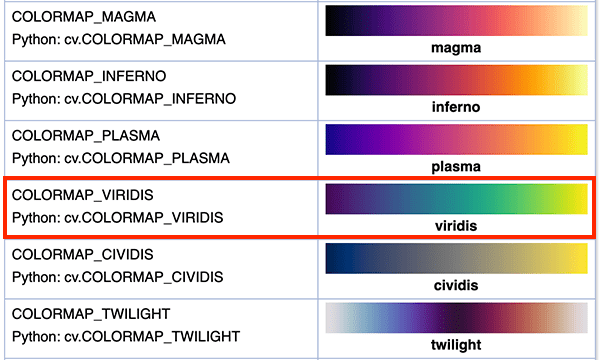
Notice how darker input grayscale values will result in a dark purple RGB color, while lighter input grayscale values will map to a light green or yellow.

Lines 93 applies the color map to the input heatmap using the VIRIDIS.

From there, we transparently overlay the heatmap on our output visualization (Line 94). The alpha channel is directly weighted into the BGR image (i.e., we are not adding an alpha channel to the image). To learn more about transparent overlays, I suggest you read my Transparent overlays with OpenCV tutorial.

Finally, Line 98 returns a 2-tuple of the heatmap (with the VIRIDIS colormap applied) along with the output visualization image.

Creating the Grad-CAM visualization script

With our Grad-CAM implementation complete, we can now move on to the driver script used to apply it for class activation mapping.

As stated previously, our apply_gradcam.py driver script accepts an image and performs inference using either a VGG16 or ResNet CNN trained on ImageNet to both (1) compute the Grad-CAM heatmap and (2) display the results in an OpenCV window.

You will be able to use this visualization script to actually “see” what is going on under the hood of your deep learning model, which many critics say is too much of a “black box” especially when it comes to public safety concerns such as self-driving cars.

Let’s dive in by opening up the apply_gradcam.py in your project structure and inserting the following code:

# import the necessary packages
from pyimagesearch.gradcam import GradCAM
from tensorflow.keras.applications import ResNet50
from tensorflow.keras.applications import VGG16
from tensorflow.keras.preprocessing.image import img_to_array
from tensorflow.keras.preprocessing.image import load_img
from tensorflow.keras.applications import imagenet_utils
import numpy as np
import argparse
import imutils
import cv2

# construct the argument parser and parse the arguments
ap = argparse.ArgumentParser()
ap.add_argument("-i", "--image", required=True,
	help="path to the input image")
ap.add_argument("-m", "--model", type=str, default="vgg",
	choices=("vgg", "resnet"),
	help="model to be used")
args = vars(ap.parse_args())

This script’s most notable imports are our GradCAM implementation, ResNet/VGG architectures, and OpenCV.

Our script accepts two command line arguments:

• --image: The path to our input image which we seek to both classify and apply Grad-CAM to.
• --model: The deep learning model we would like to apply. By default, we will use VGG16 with our Grad-CAM. Alternatively, you can specify ResNet50. Your choices in this example are limited to vgg or resenet entered directly in your terminal when you type the command, but you can modify this script to work with your own architectures as well.

Given the --model argument, let’s load our model:

# initialize the model to be VGG16
Model = VGG16

# check to see if we are using ResNet
if args["model"] == "resnet":
	Model = ResNet50

# load the pre-trained CNN from disk
print("[INFO] loading model...")
model = Model(weights="imagenet")

Lines 23-31 load either VGG16 or ResNet50 with pre-trained ImageNet weights.

Alternatively, you could load your own model; we’re using VGG16 and ResNet50 in our example and for the sake of simplicity.

Next, we’ll load and preprocess our --image:

# load the original image from disk (in OpenCV format) and then
# resize the image to its target dimensions
orig = cv2.imread(args["image"])
resized = cv2.resize(orig, (224, 224))

# load the input image from disk (in Keras/TensorFlow format) and
# preprocess it
image = load_img(args["image"], target_size=(224, 224))
image = img_to_array(image)
image = np.expand_dims(image, axis=0)
image = imagenet_utils.preprocess_input(image)

Given our input image (provided via command line argument), Line 35 loads it from disk in OpenCV BGR format while Line 40 loads the same image in TensorFlow/Keras RGB format.

Our first pre-processing step resizes the image to 224×224 pixels (Line 36 and Line 40).

If at this stage we inspect the .shape of our image , you’ll notice the shape of the NumPy array is (224, 224, 3) — each image is 224 pixels wide and 224 pixels tall, and has 3 channels (one for each of the Red, Green, and Blue channels, respectively).

However, before we can pass our image through our CNN for classification, we need to expand the dimensions to be (1, 224, 224, 3).

Why do we do this?

When classifying images using Deep Learning and Convolutional Neural Networks, we often send images through the network in “batches” for efficiency. Thus, it’s actually quite rare to pass only one image at a time through the network — unless of course, you only have one image to classify and apply Grad-MAP to (like we do).

Thus, we convert the image to an array and add a batch dimension (Lines 41 and 42).

We then preprocess the image on Line 43 by subtracting the mean RGB pixel intensity computed from the ImageNet dataset (i.e., mean subtraction).

For the purposes of classification (i.e., not Grad-CAM yet), next we’ll make predictions on the image with our model:

# use the network to make predictions on the input image and find
# the class label index with the largest corresponding probability
preds = model.predict(image)
i = np.argmax(preds[0])

# decode the ImageNet predictions to obtain the human-readable label
decoded = imagenet_utils.decode_predictions(preds)
(imagenetID, label, prob) = decoded[0][0]
label = "{}: {:.2f}%".format(label, prob * 100)
print("[INFO] {}".format(label))

Line 47 performs inference, passing our image through our CNN.

We then find the class label index with largest corresponding probability (Lines 48-53).

Alternatively, you could hardcode the class label index you want to visualize for if you believe your model is struggling with a particular class label and you want to visualize the class activation mappings for it.

At this point, we’re ready to compute our Grad-CAM heatmap visualization:

# initialize our gradient class activation map and build the heatmap
cam = GradCAM(model, i)
heatmap = cam.compute_heatmap(image)

# resize the resulting heatmap to the original input image dimensions
# and then overlay heatmap on top of the image
heatmap = cv2.resize(heatmap, (orig.shape[1], orig.shape[0]))
(heatmap, output) = cam.overlay_heatmap(heatmap, orig, alpha=0.5)

To apply Grad-CAM, we instantiate a GradCAM object with our model and highest probability class index, i (Line 57).

Then we compute the heatmap — the heart of Grad-CAM lies in the compute_heatmap method (Line 58).

We then scale/resize the heatmap to our original input dimensions and overlay the heatmap on our output image with 50% alpha transparency (Lines 62 and 63).

Finally, we produce a stacked visualization consisting of (1) the original image, (2) the heatmap, and (3) the heatmap transparently overlaid on the original image with the predicted class label:

# draw the predicted label on the output image
cv2.rectangle(output, (0, 0), (340, 40), (0, 0, 0), -1)
cv2.putText(output, label, (10, 25), cv2.FONT_HERSHEY_SIMPLEX,
	0.8, (255, 255, 255), 2)

# display the original image and resulting heatmap and output image
# to our screen
output = np.vstack([orig, heatmap, output])
output = imutils.resize(output, height=700)
cv2.imshow("Output", output)
cv2.waitKey(0)

Lines 66-68 draw the predicted class label on the top of the output Grad-CAM image.

We then stack our three images for visualization, resize to a known height that will fit on our screen, and display the result in an OpenCV window (Lines 72-75).

In the next section, we’ll apply Grad-CAM to three sample images and see if the results meet our expectations.

Visualizing class activation maps with Grad-CAM, Keras, and TensorFlow

To use Grad-CAM to visualize class activation maps, make sure you use the “Downloads” section of this tutorial to download our Keras and TensorFlow Grad-CAM implementation.

From there, open up a terminal, and execute the following command:

$ python apply_gradcam.py --image images/space_shuttle.jpg
[INFO] loading model...
[INFO] space_shuttle: 100.00%

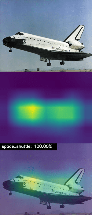
Here you can see that VGG16 has correctly classified our input image as space shuttle with 100% confidence — and by looking at our Grad-CAM output in Figure 4, we can see that VGG16 is correctly activating around patterns on the space shuttle, verifying that the network is behaving as expected.

Let’s try another image:

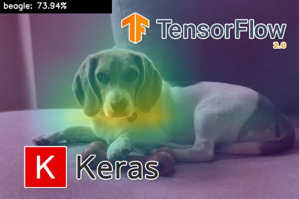
$ python apply_gradcam.py --image images/beagle.jpg
[INFO] loading model...
[INFO] beagle: 73.94%

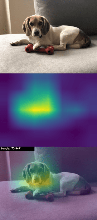
This time, we are passing in an image of my dog, Janie. VGG16 correctly labels the image as beagle.

Examining the Grad-CAM output in Figure 5, we can see that VGG16 is activating around the face of Janie, indicating that my dog’s face is an important characteristic used by the network to classify her as a beagle.

Let’s examine one final image, this time using the ResNet architecture:

$ python apply_gradcam.py --image images/soccer_ball.jpg --model resnet
[INFO] loading model...
[INFO] soccer_ball: 99.97%

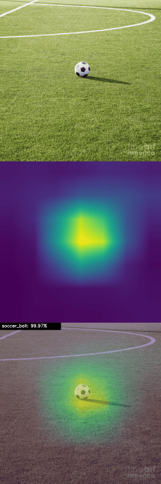
Our soccer ball is correctly classified with 99.97% accuracy, but what is more interesting is the class activation visualization in Figure 6 — notice how our network is effectively ignoring the soccer field, activating only around the soccer ball.

This activation behavior verifies that our model has correctly learned the soccer ball class during training.

After training your own CNNs, I would strongly encourage you to apply Grad-CAM and visually verify that your model is learning the patterns that you think it learning (and not some other pattern that occurs by happenstance in your dataset).

Summary

In this tutorial, you learned about Grad-CAM, an algorithm that can be used to visualize class activation maps and debug your Convolutional Neural Networks, ensuring that your network is “looking” at the correct locations in an image.

Keep in mind that if your network is performing well on your training and testing sets, there is still a chance that your accuracy resulted by accident or happenstance!

Your “high accuracy” model may be activating under patterns you did not notice or perceive in the image dataset.

I would suggest you make a conscious effort to incorporate Grad-CAM into your own deep learning pipelines and visually verify that your model is performing correctly.

The last thing you want to do is deploy a model that you think is performing well but in reality is activating under patterns irrelevant to the objects in images you want to recognize.

To download the source code to this post (and be notified when future tutorials are published here on PyImageSearch), just enter your email address in the form below!