In this tutorial, you will learn how to use OpenCV’s basic drawing functions. You will learn how to use OpenCV to draw:
- Lines
- Rectangles
- Circles
You will also learn how to use OpenCV to draw on images and blank/empty arrays initialized with NumPy.
To learn how to use OpenCV’s basic drawing functions, just keep reading.
Drawing with OpenCV
In the first part of this tutorial, we will briefly review OpenCV’s drawing functions.
We will then configure our development environment and review our project directory structure.
With the review taken care of, we will move on to implement two Python scripts:
basic_drawing.pyimage_drawing.py
These scripts will help you understand how to perform basic drawing functions with OpenCV.
By the end of this guide, you will understand how to use OpenCV to draw lines, circles, and rectangles.
Drawing functions in OpenCV
OpenCV has a number of drawing functions you can use to draw various shapes, including polygons of irregular shapes, but the three most common OpenCV drawing functions you will see are:
cv2.line: Draws a line on image, starting at a specified (x, y)-coordinate and ending at another (x, y)-coordinatecv2.circle: Draws a circle on an image specified by the center (x, y)-coordinate and a supplied radiuscv2.rectangle: Draws a rectangle on an image specified by the top-left corner and bottom-right corner (x, y)-coordinates
We will cover these three drawing functions today.
However, it’s worth noting that more advanced OpenCV drawing functions exist, including:
cv2.ellipse: Draws an ellipse on an imagecv2.polylines: Draws the outline of a polygon specified by a set of (x, y)-coordinatescv2.fillPoly: Draws a polygon, but instead of drawing the outline, instead fills in the polygoncv2.arrowedLine: Draws an arrow pointing from a starting (x, y)-coordinate to an ending (x, y)-coordinate
These OpenCV drawing functions are used less often but are still worth noting. We use them occasionally on the PyImageSearch blog.
Configuring your development environment
To follow along with this guide, you need to have the OpenCV library installed on your system.
Luckily, OpenCV is pip-installable:
$ pip install opencv-contrib-python
If you need help configuring your development environment for OpenCV, I highly recommend that you read my pip install OpenCV guide — it will have your system up and running in a matter of minutes.
Having problems configuring your development environment?
All that said, are you:
- Short on time?
- Learning on your employer’s administratively locked system?
- Wanting to skip the hassle of fighting with the command line, package managers, and virtual environments?
- Ready to run the code right now on your Windows, macOS, or Linux systems?
Then join PyImageSearch Plus today!
Gain access to Jupyter Notebooks for this tutorial and other PyImageSearch guides that are pre-configured to run on Google Colab’s ecosystem right in your web browser! No installation required.
And best of all, these Jupyter Notebooks will run on Windows, macOS, and Linux!
Project structure
Let’s start by reviewing our project directory structure for our OpenCV drawing project:
$ tree . --dirsfirst
.
├── adrian.png
├── basic_drawing.py
└── image_drawing.py

0 directories, 3 files
We have two Python scripts to review today:
basic_drawing.py: Initializes an empty NumPy array and utilizes OpenCV to draw lines, circles, and rectanglesimage_drawing.py: Loadsadrian.pngfrom disk and then draws on the image (rather than an empty/blank NumPy array canvas).
We are now ready to get started!
Implementing basic drawing functions with OpenCV
Before we draw on actual images, let’s first learn how to initialize an empty NumPy array/image and draw on it.
Open the basic_drawing.py file in your project directory structure, and let’s get to work.
# import the necessary packages
import numpy as np
import cv2

# initialize our canvas as a 300x300 pixel image with 3 channels
# (Red, Green, and Blue) with a black background
canvas = np.zeros((300, 300, 3), dtype="uint8")
Lines 2 and 3 import the packages we will be using.
As a shortcut, we will create an alias for numpy as np. You will see this convention utilized in all PyImageSearch tutorials that leverage NumPy (and in fact, you will commonly see this convention in the Python community as well!)
We will also import cv2, so we can have access to the OpenCV library.
Initializing our image is handled on Line 7. We construct a NumPy array using the np.zeros method with 300 rows and 300 columns, yielding a 300 x 300 pixel image. We also allocate space for 3 channels — one each for Red, Green, and Blue. As the name suggests, the np.zeros method fills every element in the array with an initial value of zero.
Secondly, it’s important to draw your attention to the second argument of the np.zeros method: the data type, dtype.
Since we represent our image as an RGB image with pixels in the range [0, 255], we must use an 8-bit unsigned integer, or uint8. There are many other data types that we can use (common ones include 32-bit integers and 32- and 64-bit floats), but we will mainly use uint8 for the majority of the examples in this lesson.
Now that we have our canvas initialized, we can do some drawing:
# draw a green line from the top-left corner of our canvas to the
# bottom-right
green = (0, 255, 0)
cv2.line(canvas, (0, 0), (300, 300), green)
cv2.imshow("Canvas", canvas)
cv2.waitKey(0)

# draw a 3 pixel thick red line from the top-right corner to the
# bottom-left
red = (0, 0, 255)
cv2.line(canvas, (300, 0), (0, 300), red, 3)
cv2.imshow("Canvas", canvas)
cv2.waitKey(0)
The first thing we do on Line 11 is to define a tuple used to represent the color “green.” Then, we draw a green line from point (0, 0), the top-left corner of the image, to point (300, 300), the bottom-right corner of the image, on Line 12.
In order to draw the line, we make use of the cv2.line method:
- The first argument to this method is the image upon which we are going to draw. In this case, it’s our
canvas. - The second argument is the starting point of the line. We choose to start our line from the top-left corner of the image, at point (0, 0) — again, remember that the Python language is zero-index.
- We also need to supply an ending point for the line (the third argument). We define our ending point to be (300, 300), the bottom-right corner of the image.
- The last argument is the color of our line (in this case, green). Lines 13 and 14 show our image and then wait for a keypress (see Figure 2).
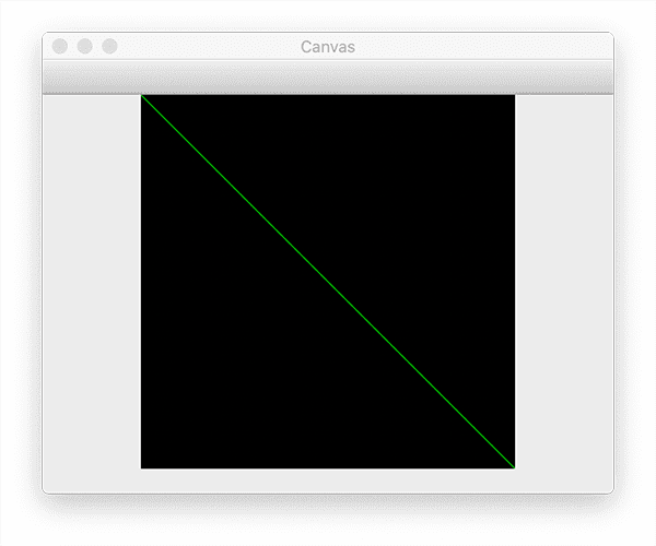
As you can see, using the cv2.line function is quite simple! But there is one other important argument to consider in the cv2.line method: the thickness.
On Lines 18-21, we define the color red as a tuple (again, in BGR rather than RGB format). We then draw a red line from the top-right corner of the image to the bottom-left. The last parameter to the method controls the thickness of the line — we decide to make the thickness 3 pixels. Again, we show our image and wait for a keypress:
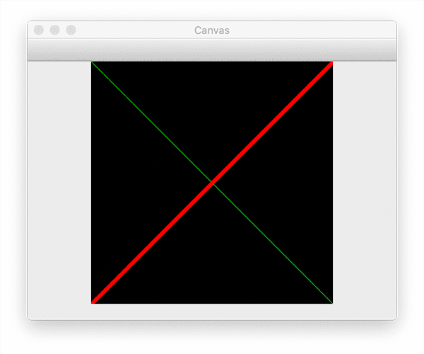
Drawing a line was simple enough. Now we can move on to drawing rectangles. Check out the code below for more details:
# draw a green 50x50 pixel square, starting at 10x10 and ending at 60x60
cv2.rectangle(canvas, (10, 10), (60, 60), green)
cv2.imshow("Canvas", canvas)
cv2.waitKey(0)

# draw another rectangle, this one red with 5 pixel thickness
cv2.rectangle(canvas, (50, 200), (200, 225), red, 5)
cv2.imshow("Canvas", canvas)
cv2.waitKey(0)

# draw a final rectangle (blue and filled in )
blue = (255, 0, 0)
cv2.rectangle(canvas, (200, 50), (225, 125), blue, -1)
cv2.imshow("Canvas", canvas)
cv2.waitKey(0)
On Line 24, we make use of the cv2.rectangle method. The signature of this method is identical to the cv2.line method above, but let’s explore each argument anyway:
- The first argument is the image upon which we want to draw our rectangle. We want to draw on our
canvas, so we pass it into the method. - The second argument is the starting (x, y) position of our rectangle — here, we start our rectangle at point (10, 10).
- Then, we must provide an ending (x, y) point for the rectangle. We decide to end our rectangle at (60, 60), defining a region of 50 x 50 pixels (take a second to convince yourself that the resulting rectangle is 50 x 50).
- Finally, the last argument is the color of the rectangle we want to draw. Here, we are drawing a green rectangle.
Just as we can control a line’s thickness, we can also control the rectangle’s thickness. Line 29 provides that thickness argument. Here, we draw a red rectangle that is 5 pixels thick, starting at point (50, 200) and ending at (200, 225).
At this point, we have only drawn the outline of a rectangle. How do we draw a rectangle that is “completely filled”?
Simple. We just pass a negative value for the thickness argument.
Line 35 demonstrates how to draw a rectangle of a solid color. We draw a blue rectangle, starting at (200, 50) and ending at (225, 125). By specifying -1 (or use the cv2.FILLED keyword) as the thickness, our rectangle is drawn as a solid blue.
Figure 4 displays the full output of drawing our lines and rectangles:
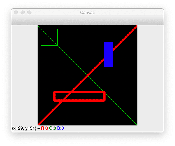
As you can see, the output matches our code. We could draw a green line from the top-left corner to the bottom-right corner, followed by a thicker red line from the top-right corner to the bottom-left corner.
We were also able to draw a green rectangle, a slightly thicker red rectangle, and a completely filled blue rectangle.
That’s great and all — but what about circles?
How can we use OpenCV to draw circles?
Drawing circles is just as simple as drawing rectangles, but the function arguments are a little different:
# re-initialize our canvas as an empty array, then compute the
# center (x, y)-coordinates of the canvas
canvas = np.zeros((300, 300, 3), dtype="uint8")
(centerX, centerY) = (canvas.shape[1] // 2, canvas.shape[0] // 2)
white = (255, 255, 255)

# loop over increasing radii, from 25 pixels to 150 pixels in 25
# pixel increments
for r in range(0, 175, 25):
	# draw a white circle with the current radius size
	cv2.circle(canvas, (centerX, centerY), r, white)

# show our work of art
cv2.imshow("Canvas", canvas)
cv2.waitKey(0)
On Line 41, we re-initialize our canvas to blank:
Line 42 calculates two variables: centerX and centerY. These two variables represent the (x, y)-coordinates of the image’s center.
We calculate the center by examining the shape of our NumPy array and then dividing by two:
- The height of the image can be found in
canvas.shape[0](number of rows) - The width is found in
canvas.shape[1](number of columns)
Finally, Line 43 defines a white pixel (i.e., the buckets for each of the Red, Green, and Blue components are “full”).
Now, let’s draw some circles!
On Line 45, we loop over several radius values, starting at 0 and ending at 150, incrementing by 25 at each step. The range function is exclusive; therefore, we specify a stopping value of 175 rather than 150.
To demonstrate this for yourself, open a Python shell, and execute the following code:
$ python
>>> list(range(0, 175, 25))
[0, 25, 50, 75, 100, 125, 150]
Notice how the output of range stops at 150 and does not include 175.
Line 49 handles the actual drawing of the circle:
- The first parameter is our
canvas, the image upon which we want to draw the circle. - We then need to supply the point around which we will draw our circle. We pass in a tuple of
(centerX, centerY)so that our circles will be centered at the center of the image. - The third argument is the radius,
r, of the circle we wish to draw. - Finally, we pass in the color of our circle: in this case, white.
Lines 52 and 53 then show our image and wait for a keypress:
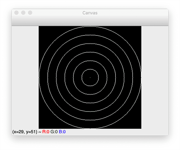
Check out Figure 6, and you will see that we have drawn a simple bullseye! The “dot” in the very center of the image is drawn with a radius of 0. The larger circles are drawn with ever-increasing radii sizes from our for loop.
Not too bad. But what else can we do?
Let’s do some abstract drawing:
# re-initialize our canvas once again
canvas = np.zeros((300, 300, 3), dtype="uint8")

# let's draw 25 random circles
for i in range(0, 25):
	# randomly generate a radius size between 5 and 200, generate a
	# random color, and then pick a random point on our canvas where
	# the circle will be drawn
	radius = np.random.randint(5, high=200)
	color = np.random.randint(0, high=256, size=(3,)).tolist()
	pt = np.random.randint(0, high=300, size=(2,))

	# draw our random circle on the canvas
	cv2.circle(canvas, tuple(pt), radius, color, -1)

# display our masterpiece to our screen
cv2.imshow("Canvas", canvas)
cv2.waitKey(0)
Our code starts on Line 59 with more looping. This time we aren’t looping over our radii’s size — we are instead going to draw 25 random circles, making use of NumPy’s random number capabilities through the np.random.randint function.
To draw a random circle, we need to generate three values: the radius of the circle, the color of the circle, and the pt — the (x, y)-coordinate of where the circle will be drawn.
We generate a radius value in the range [5, 200] on Line 63. This value controls how large our circle will be.
On Line 64, we randomly generate a color. As we know, the color of an RGB pixel consists of three values in the range [0, 255]. To get three random integers rather than only one integer, we pass the keyword argument size=(3,), instructing NumPy to return a list of three numbers.
Lastly, we need an (x, y)-center point to draw our circle. We will generate a point in the range [0, 300), again using NumPy’s np.random.randint function.
The drawing of our circle then takes place on Line 68, using the radius, color, and pt that we randomly generated. Notice how we use a thickness of -1, so our circles are drawn as a solid color and not just an outline.
Lines 71 and 72 shown our masterpiece, which you can see in Figure 7:
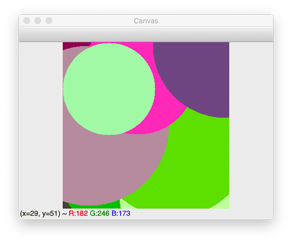
Notice how each circle has a different size, color, and placement on our canvas.
OpenCV basic drawing results
To execute our basic drawing script, be sure to access the “Downloads” section to retrieve the source code and example image.
From there, you can execute the following command:
$ python basic_drawing.py
Your output should be identical to that of the previous section.
Drawing on images with OpenCV
Up until this point, we have only explored drawing shapes on a blank canvas. But what if we want to draw shapes on an existing image?
It turns out that the code to draw shapes on an existing image is exactly the same as if we were drawing on a blank canvas generated from NumPy.
To demonstrate this, let’s look at some code:
# import the necessary packages
import argparse
import cv2

# construct the argument parser and parse the arguments
ap = argparse.ArgumentParser()
ap.add_argument("-i", "--image", type=str, default="adrian.png",
	help="path to the input image")
args = vars(ap.parse_args())
Lines 2 and 3 import our required Python packages, while Lines 6-9 parse our command line arguments.
We only need a single argument, --image, which is the path to our input image on disk. By default, we set the --image command line argument to point to the adrian.png image in our project directory structure.
# load the input image from disk
image = cv2.imread(args["image"])

# draw a circle around my face, two filled in circles covering my
# eyes, and a rectangle over top of my mouth
cv2.circle(image, (168, 188), 90, (0, 0, 255), 2)
cv2.circle(image, (150, 164), 10, (0, 0, 255), -1)
cv2.circle(image, (192, 174), 10, (0, 0, 255), -1)
cv2.rectangle(image, (134, 200), (186, 218), (0, 0, 255), -1)

# show the output image
cv2.imshow("Output", image)
cv2.waitKey(0)
Line 12 loads our --image from disk. From there, we proceed to:
- Draw an empty circle (not filled in) surrounding my head (Line 16)
- Draw two filled in circles covering my eyes (Lines 17 and 18)
- Draw a rectangle over my mouth (Line 19)
Our final output, image, is then displayed on our screen.
OpenCV image drawing results
Let’s see how we can use OpenCV to draw on an image versus a “blank canvas” generated by NumPy.
Start by accessing the “Downloads” section of this guide to retrieve the source code and example image.
You can then execute the following command:
$ python image_drawing.py

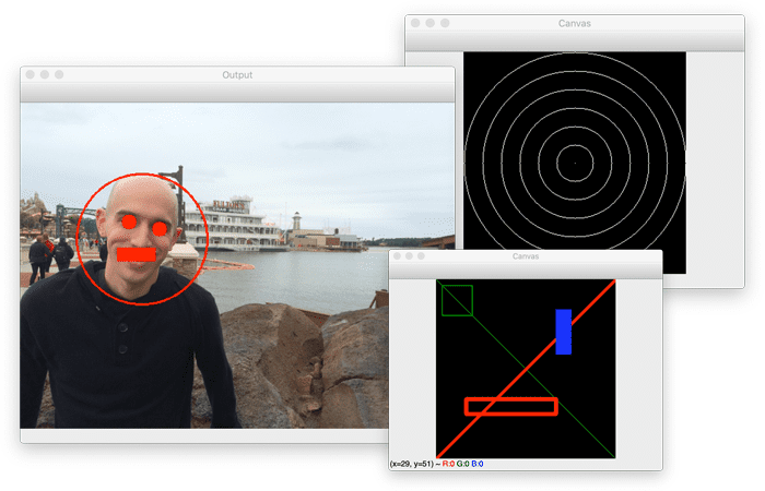
Here, you can see that we have drawn an outlined circle surrounding my face, two filled circles over my eyes, and a filled rectangle over my mouth.
In fact, there is no difference between drawing shapes on an image loaded from disk versus a blank NumPy array. As long as our image/canvas can be represented as a NumPy array, OpenCV will draw on it just the same.
What's next? I recommend PyImageSearch University.
30+ total classes • 39h 44m video • Last updated: 12/2021
★★★★★ 4.84 (128 Ratings) • 3,000+ Students Enrolled
I strongly believe that if you had the right teacher you could master computer vision and deep learning.
Do you think learning computer vision and deep learning has to be time-consuming, overwhelming, and complicated? Or has to involve complex mathematics and equations? Or requires a degree in computer science?
That’s not the case.
All you need to master computer vision and deep learning is for someone to explain things to you in simple, intuitive terms. And that’s exactly what I do. My mission is to change education and how complex Artificial Intelligence topics are taught.
If you're serious about learning computer vision, your next stop should be PyImageSearch University, the most comprehensive computer vision, deep learning, and OpenCV course online today. Here you’ll learn how to successfully and confidently apply computer vision to your work, research, and projects. Join me in computer vision mastery.
Inside PyImageSearch University you'll find:
- ✓ 30+ courses on essential computer vision, deep learning, and OpenCV topics
- ✓ 30+ Certificates of Completion
- ✓ 39h 44m on-demand video
- ✓ Brand new courses released every month, ensuring you can keep up with state-of-the-art techniques
- ✓ Pre-configured Jupyter Notebooks in Google Colab
- ✓ Run all code examples in your web browser — works on Windows, macOS, and Linux (no dev environment configuration required!)
- ✓ Access to centralized code repos for all 500+ tutorials on PyImageSearch
- ✓ Easy one-click downloads for code, datasets, pre-trained models, etc.
- ✓ Access on mobile, laptop, desktop, etc.
Summary
In this tutorial, you learned how to draw with OpenCV. Specifically, you learned how to use OpenCV to draw:
- Lines
- Circles
- Rectangles
Lines were drawn using the cv2.line function. We used the cv2.circle function to draw circles and the cv2.rectangle method to draw rectangles with OpenCV.
Other drawing functions exist in OpenCV. However, these are the functions you will use most often.
To download the source code to this post (and be notified when future tutorials are published here on PyImageSearch), simply enter your email address in the form below!

Download the Source Code and FREE 17-page Resource Guide
Enter your email address below to get a .zip of the code and a FREE 17-page Resource Guide on Computer Vision, OpenCV, and Deep Learning. Inside you'll find my hand-picked tutorials, books, courses, and libraries to help you master CV and DL!


Comment section
Hey, Adrian Rosebrock here, author and creator of PyImageSearch. While I love hearing from readers, a couple years ago I made the tough decision to no longer offer 1:1 help over blog post comments.
At the time I was receiving 200+ emails per day and another 100+ blog post comments. I simply did not have the time to moderate and respond to them all, and the sheer volume of requests was taking a toll on me.
Instead, my goal is to do the most good for the computer vision, deep learning, and OpenCV community at large by focusing my time on authoring high-quality blog posts, tutorials, and books/courses.
If you need help learning computer vision and deep learning, I suggest you refer to my full catalog of books and courses — they have helped tens of thousands of developers, students, and researchers just like yourself learn Computer Vision, Deep Learning, and OpenCV.
Click here to browse my full catalog.